What is a Signal Amplifier and How Does it Work?

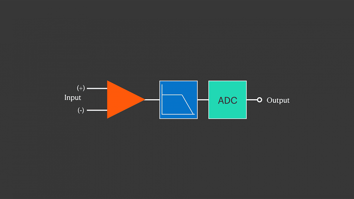
What is a signal amplifier?

A signal amplifier is a circuit that uses electrical power to increase the amplitude of an incoming signal voltage or current signal, and output this higher amplitude version at its output terminals. The ideal signal amplifier creates an exact replica of the original signal that is larger but identical in every other way. In practice, a “perfect” amplifier is not possible, because no circuit can perfectly and proportionately scale up all aspects of a signal past a certain point.

Signal amplifiers are an essential component of thousands of devices, including landline and cellular telephone systems, music and public address systems, data acquisition (DAQ) systems, radio frequency transmitters, servo motor controllers, and countless more.

In data acquisition (DAQ) systems, signal amplifiers are needed to increase the amplitudes from sensors that output small signals, up to the level where they can be sent to an A/D converter (ADC) for digitization. The typical analoge-to-digital converter has an input aperture of ±5 V. Therefore, signals from thermocouples, shunts, strain gages, et al that are far lower than ±5V must be amplified significantly before they are sent to the ADC.

Types of signal amplifiers

There are several types of signal amplifiers, each capable of conditioning different signal types. Here is a list of some common signal amplifiers found in today's data acquisition systems:

• Differential amplifiers

• Isolated amplifiers

• Voltage amplifiers: low voltage amplifier, high voltage amplifier, DC voltage amplifier, AC voltage amplifier

• Current amplifiers

• Piezoelectric amplifiers

• Charge amplifiers

• Thermocouple amplifiers

• Strain gauge amplifiers: bridge amplifier, full-bridge amplifier, half-bridge amplifier, quarter-bridge amplifier)

• Resistance amplifiers

• LVDT amplifiers

Preserving a signal’s essential characteristics

The purpose of a guitar amplifier is to take the low-level output from an electric guitar and make it sound good. It has nothing to do with accuracy (which is irrelevant in this application), and everything to do with aesthetics. We simply want a good sound from this signal amplifier, and the electronics within classic tube amps are designed intentionally to “colour” the sound to make it more pleasing within the context of a certain type of music.

However, the purpose of a DAQ system is to make accurate, objective measurements of signals. Therefore, all aspects of the system are designed to preserve signal accuracy. It would be self-defeating if a DAQ system distorted the character and nature of the signal when it increased the signal’s amplitude. Again, the ideal signal amplifier should not distort the original signal in any way. So how can we achieve this?

Very strong clues about which elements of a signal are most essential to be preserved can be observed by a quick look at the specifications of the signal amplifiers (aka “signal conditioners”) used in today’s best DAQ systems. Here are the elements that are most often specified:

• Input Ranges

• Bandwidth and “Alias-free” Bandwidth

• Sampling Rate

• Gain Accuracy

• Gain Drift

• Gain Linearity

• Offset Accuracy

• Offset Drift

• Dynamic Range

• Noise Floor

• Input Impedance

• Maximum Common-Mode Voltage

• Isolation

Let’s take a look at each one of these specifications and see how they work within DAQ signal amplifiers.

What is input range?

Input ranges are the selectable input gains that can be applied to the signal. In a typical low-voltage signal conditioner, these might range from ±100 mV to ±50 V (or higher), with several steps in between. 

The user selects the input range that best matches the signal’s total bipolar amplitude. So for example, if a signal is ranging around (but not exceeding) ±500 mV, a ±500 mV input range setting would be ideal. If this is not available in the DAQ system, the user should choose the next higher-up range, for example, ±1V. 

It is important that the signal does not exceed either of the maximum bipolar limits of the selected input range, to avoid “clipping” the extremes of the signal.

The job of the signal conditioner is to then amplify each of these ranges to the ideal ±5 V output that the ADC requires. Therefore, a ±5V input range would mean unity gain, or a 1:1 ratio between input and output, whereas selecting a ±500 mV input range would mean that the amplifier has a gain of 10:1. Selecting a ±200V range would mean a gain of 1:40 - i.e., an attenuation of 40 to 1. Regardless of the range, the output is scaled to the ideal ±5 V for presenting to the ADC.

At this point, it should be obvious that our DAQ system’s signal “amplifier” also has to be a signal “reducer,” depending on the input range that the user has selected. It has to perform equally well regardless of whether it is amplifying the signal, attenuating it, or neither (unity gain).

What if the wrong range is selected? Well, if the user selects a range that is too large, the signal will be very small within the ±5 V output aperture. The result will be less resolution when digitized and a poor signal-to-noise ratio. 

Using a range that’s too large is like standing 200 feet away and taking a picture of a cat with a regular camera... There will be relatively few pixels containing a cat in the resulting image. Move closer until the cat fills the frame, and the entire resolution of the camera is used to capture the cat.

On the other hand, if you stand too close you can only take a picture of part of the cat, right? Parts of the cat will not be in the frame at all. The same thing happens if the user chooses an input range that is too small for the signal: part of the signal will be “clipped” and not recorded at all.

OK, we’re not measuring cats, but you get the idea: selecting the correct input range is critical to achieving the best possible signal-to-noise ratio and signal resolution and avoiding “clipped” aka over-modulated measurements.

The solution to wrong input range settings - Dewesoft DualCoreADC® technology

Engineers have struggled for years with this quandary. They want to select a range that will provide them with the best possible resolution, but some signals are unpredictable and will increase in amplitude during a measurement far beyond what was expected. 

One solution would be to input each signal into two different input channels on the DAQ system:

• One channel is set for the best resolution for most of the tests. 

• The other channel is set at a larger range for those times when the signal dramatically increases in amplitude.

This would work, but it is very inefficient: using two channels for every input signal would require twice as many DAQ systems in order to do the same work. In addition, it would make data analysis after each test much more complex and time-consuming. 

Dewesoft’s DualCoreADC® technology solves this problem by using two separate 24-bit ADCs per channel, automatically switching between them in real-time and creating a single, seamless channel. These two ADCs always measure the high and low gain of the input signal. This results in the full possible measuring range of the sensor and prevents the signal from being clipped.

And it’s not just for dynamic signals: even with very slow signals like from most thermocouples, having the greatest possible amplitude axis resolution can be critical.

Imagine a thermocouple capable of measuring across a 1500° span. Most of the time it’s within a hundred degrees or so, but occasionally it will rise up to 800° or more. Even with this very slow signal, DualCoreADC® technology is a big advantage, because it automatically switches between Gain1 for most of the signal and Gain2 during high amplitude excursions, preserving optimal Y-axis resolution at all times.

With DualCoreADC® technology SIRIUS DAQ systems achieve more than 130 dB signal-to-noise ratio and more than 160 dB in dynamic range. This is 20 times better than typical 24-bit systems with 20 times less noise.

What are bandwidth and alias-free bandwidth?

Also called “frequency response,” bandwidth is the range of frequencies within which a signal amplifier’s performance is thought to be satisfactory. This has historically been accepted to mean that it can reproduce the signal up to the point where the signal’s amplitude is still within -3 dB of its true value. This so-called “3 dB point” can also be expressed as the signal at 70.7% of its true amplitude.

Let’s look at a real-world example with the SIRIUS LV (low voltage) signal amplifier. The rated bandwidth of this model is 70 kHz. In part, this is because the SIRIUS LV is not a stand-alone signal conditioner, but has a fully integrated ADC as well. In fact, this is a delta-sigma ADC with 24-bit resolution and built-in anti-aliasing filtering.

One of the characteristics of delta-sigma ADCs is that they sample much faster than the selected rate. They use powerful DSP electronics onboard to derive an output data stream with very high amplitude axis resolution, in this case, 24 bits. This scheme also prevents aliased (i.e., “false”) signals caused by sampling too slowly for the incoming signals. 

As a result, the bandwidth is also the “alias-free” bandwidth, meaning that aliased signals are not possible within this range. Signal amplifiers that do not also incorporate A/D conversion cannot specify the alias-free bandwidth, because this specification is related to the A/D process.

To achieve the best possible bandwidth and anti-aliasing results, a combination of technologies is used:

• analog filtering,

• oversampling, and

• digital filtering.

Looking at the chart above, you can see that the orange line representing the SIRIUS filtering is almost perfect. So how was this achieved? It is well-known that every filter imposes a phase shift, so how is this possible?

To achieve a very sharp roll-off (“damping”) we need a high-order filter. This leads us to filter in the digital domain as opposed to the analog, however, digital filtering cannot be used to prevent aliasing. You can learn more about this in the What is an A/D converter.

Therefore, by first filtering in the analog domain to block aliasing, and then filtering in the digital domain, this is possible. But for the best phase results, we should use an FIR (Finite Infinite Response) filter, one of the most demanding computations among filtering, requiring a lot of processing power. 

Luckily, the DSP within the SIRIUS ADC subsystem is capable of the millions of calculations per second required. In addition, its delta-sigma architecture includes over-sampling, which raises the Nyquist frequency and improves signal quality. The result is a very steep roll-off at a predictable frequency, in this case, 70 kHz.

It should be noted that there are other SIRIUS signal amplifiers, such as the HS (high speed) series that use a faster A/D and thus offer a higher bandwidth and alias-free bandwidth. Depending on the specific module, the HS series offers bandwidths of 500 kHz, 1 MHz, and 2 MHz. In addition, the SIRIUS XHS series offers bandwidth up to 5 MHz in the high bandwidth mode.

In all cases, it is important to match the instrument with the application. For nearly every DAQ measurement within the physical (electrical and mechanical) domain, the bandwidth offered by the SIRIUS series of signal amplifiers is more than adequate.

What is the sampling rate (sample rate)?

When specifying a DAQ system most people look at the sample rate as the top speed of a car. “How fast can this thing go?”

It’s an important question, of course, but we also have to consider the effective bandwidth and alias-free bandwidth of the system (see the previous section), which is why that specification is perhaps more important.

The sample rate is simply the speed or rate at which the A/D converter within a DAQ system can sample the incoming analog data from the signal amplifier. It is clearly related to the bandwidth that we discussed above.

If we continue using SIRIUS as our example, these modules are available in two varieties:

• SIRIUS DualCore and HD (High Density): Maximum sample rate: 200 kS/s/ch

• SIRIUS HS (High Speed): Maximum sample rate: 1 MS/s/ch

• SIRIUS XHS (eXtra High Speed): Maximum sample rate: 15 MS/s/ch

Where:

All channels are sampled simultaneously, so if we are recording 8 channels at 1 MS/s/ch then 8 million samples are being written to disk per second. It is common practice to use the term “samples” to mean a word of data, as opposed to “bytes” because a sample is more than one byte. In a 16-bit system, a sample is two bytes, but in a 24-bit system, it is four bytes. So it’s more useful and less confusing to use the term “samples.”

So while the sample rate is not specifically related to the analog part of the signal amplifier itself, in the case of SIRIUS with its built-in ADC system, it is a valid concern because of the tight integration of the analog and digital elements of the signal chain. As shown earlier, these sections have been designed as a single system in order to achieve the best possible performance.

What is gain accuracy?

Gain accuracy is the accuracy at which a signal amplifier can amplify a signal. For example, if we have a 1.287 V incoming signal and we ask our amplifier to increase its amplitude by a factor of 10, the amplifier should give us an output signal of 12.870 V: exactly 10 times larger, in this example. The difference between the ideal amplification and the actual amplification is the gain error. 

The ideal signal amplifier would have no gain error at all, but in reality, there is some error in every system.

Gain accuracy can also be expressed in terms of “gain error,” which is simply the inverse of gain accuracy.

Common abbreviations for this metric include “% FS” for a percentage of full scale and “% RD” for a percentage of reading.

Gain error is a magnitude measurement expressed normally as a percentage of the actual signal reading. But it can also be given as a percentage of full-scale, which can be very different. How?

Using an example with round numbers - consider these two hypothetical systems: they each specify the gain accuracy of their 10V range to be 1%. 

Hypothetical system A specifies gain error at reading, while hypothetical system B specifies it at full scale. What’s the difference?

To test it we insert exactly the same 10V signal into both systems. When the signal is at 10V and our range is 10V, the gain error should be identical in Systems A and B.

But ... what if we reduce the amplitude of the signal to 5V, what happens?

System A has a 1% gain error in the reading, so the gain error percentage follows the amplitude of the reading and remains constant. No matter what the signal is within this range, the gain error does not change - it’s always the same percentage of the signal reading.

System B has a 1% gain error regardless of the reading, therefore when the signal amplitude is reduced by 50% but the range remains at 10V, the error is doubled. If we further lower the signal to 1V the gain error could be 10 times worse than 1%, or 10%.

This is why it is important to look at how gain is actually specified.

The SIRIUS LV module has a gain accuracy specification of ±0.05% of reading. This means that no matter what the signal amplitude is within a given range, the gain accuracy (error) will not change.

What is gain drift?

Gain drift is more properly called “Gain Temperature Drift” because it is the amount of gain error that might be induced as a result of changes in the ambient temperature. Gain drift is therefore normally expressed as the number of parts per million per degree change in temperature. 

The temperature is expressed either in Celsius or in the SI unit K (Kelvin). Note that although their zero or reference points are drastically different, Kelvin and Celcius have the same magnitude. So one Celsius degree is the same magnitude as one Kelvin unit.

The SIRIUS LV signal amplifier is a good example of this specification. Its gain drift is specified as:

• Typical 10 ppm/K, max. 30 ppm/K

So in this case, two specifications are provided: the typical drift expected under everyday operating conditions, and the worst-case (maximum) drift which might be experienced under extreme conditions. The typical drift would be 10 parts per million per Kelvin unit (essentially the same as “per degree C”), in this case. 

“Parts per million” defines the fraction that the gain will deviate when subjected to a change in operating temperature. 

Another way you might see gain drift specified is like this:

• ±20 ppm/K ±100μV/K

In this case, the ppm drift per degree is specified plus an additional voltage (100 µV in this example) per degree C has to be added together to determine the maximum gain drift per degree C of temperature change. 

Of course, we need to know where we are starting with the temperature, so manufacturers normally provide the baseline operating temperature or range of operating temperatures of the instrument in question.

What is gain linearity?

Linearity refers to how well an amplifier can output amplified signals that are accurate copies of the signals that we put into it. No amplifier is perfect, of course, but a linear amplifier is designed specifically to handle this challenge. DAQ systems are in the business of making accurate measurements, so it would hardly do for their signal conditioners to fundamentally change the nature of the signals that it’s measuring.

We want our amplifier to make as perfect a copy of the original signal as possible, but simply at a different amplitude. The congruency of the incoming and outgoing waveshapes should be identical, give or take a very small amount of distortion or “non-linearity.".

Using the SIRIUS LV signal conditioner as an example, this module has a gain linearity specification of <0.02%, which simply means that the linearity of the amplified signal compared with the original waveshape can be wrong only within 0.02%.

What is offset accuracy?

Unlike gain accuracy, which relates more to the magnitude of the signal being amplified, offset accuracy is related to the accurate Y-axis positioning of the baseline of the signal. 

Let’s use an example of a simple AC sinus waveform at ±1.000 V. This signal’s centerline is exactly at 0.000 V. If our signal conditioner is set to amplify this sine wave up to ±5.000 V, we still want our baseline to be at 0.000 V, right? Offset accuracy defines how well our signal conditioner can MAINTAIN the baseline of the signals that it amplifies.

In the case of the SIRIUS LV, the offset accuracy specification is given both before and after the built-in balanced amp. Due to the very wide range of this amplifier, the specifications are a little different depending on the range.

• In the most sensitive range of ±100 mV, the offset accuracy is ± 0.1 mV.

• In the least sensitive range of ±200 V, the offset accuracy is ± 40 mV.

So these values are absolute ones, like the ±0.1 mV offset accuracy when the ±100 mV range is selected. That’s a very impressive number, which at first glance makes the 40 mV offset accuracy specification below it seem much worse. But it is not - because that value is at the ±200 V range, which is 2000 times larger than the ±100 mV range!

What is offset drift?

As with the gain drift specification that we discussed earlier, offset drift is the tendency for this parameter to change over time based on changes in the ambient operating temperature.

Using the SIRIUS LV signal conditioner as our example, the offset drift is specified as:

• Typical 0.3 μV/K + 5ppm of range/K, max: 2 μV/k + 10 ppm of range/K

Again, two specifications are actually provided here: the typical drift in a normal operating environment, and the maximum drift when the system is being used in an extreme operating environment.

So in the typical operating environment, the offset drift specification is:

• 0.3 µV (0.000003 V) per Kelvin unit PLUS 5 ppm (0.000005) of the selected RANGE per Kelvin unit

What is dynamic range?

Dynamic range is perhaps easiest explained using music. One of the advantages of the music CD when it was introduced compared with vinyl records and cassette tapes, was its dynamic range. Basically, this is simply the difference between the softest and loudest sounds that the medium could express. 

Audio volume is logarithmic in nature, so dynamic range is expressed in decibels (dB).

While a cassette tape could reach 50 - 60 dB of dynamic range, and 33-⅓ RPM vinyl LP offered a dynamic range of 55 - 70 dB, music on a CD could reach as high as 96 dB, and even higher using noise-shaping to the human ear.

Dynamic range is the ratio between the largest magnitude undistorted signal and the smallest magnitude signal. To measure this in a way that can be repeated across systems, a signal like a pure sine wave at 1 kHz and a fixed magnitude like 1.228 VRMS is injected as a known reference.  

In the case of the SIRIUS LV the dynamic range specification is given for each user-selectable range at a 10 kS/s sample rate:

• In the most sensitive range of ±100 mV, the dynamic range is 130 dB

• In the least sensitive range of ±200 V, the dynamic range is 136 dB

So how does Dewesoft achieve such a high dynamic range? Ordinary DAQ systems have dynamic range specifications below 100 dB. 

The first explanation is the use of 24-bit delta-sigma ADC technology. The music CD mentioned above is a standard from the 1980s that allows only 16-bit music to be stored on the CD. If you consider that every single bit that we add to the resolution doubles the number of values that can be expressed, it is clear that 24-bit ADCs provide vastly more quantization than 16-bit ADCs.

But that is just the beginning because even other DAQ systems with similar 24-bit ADCs do not achieve these specifications. Dewesoft’s DualCoreADC® technology uses two separate 24-bit ADCs per channel, and automatically switches between them in real time, creating a single, seamless channel. These two ADCs always measure the high and low gain of the input signal. This results in the full possible measuring range of the sensor and prevents the signal from being clipped.

With DualCoreADC® technology SIRIUS achieves more than 130 dB signal-to-noise ratio and more than 160 dB in dynamic range. This is 20 times better than typical 24-bit systems with 20 times less noise.

What is the signal-to-noise ratio (SNR)?

As the name implies, this is the ratio between useful signal content, and the background or unwanted signal content  (noise) that has crept into the signal chain. Signal to noise (often abbreviated as S/N or SNR) is expressed in decibels (dB)

This specification is closely related to the dynamic range described above. Dewesoft DualCoreADC technology dramatically improves the signal-to-noise ratio of SIRIUS measuring systems by use of two independent 24-bit ADCs set to two different gain apertures and then combining their streams into a single stream with the lowest possible noise floor and best possible dynamic range and signal to noise ratio.

What is noise floor?

Closely related to the Signal to Noise ratio described above, the “noise floor” is simply the sum of all unwanted signals, called “noise,” that is present within a measurement system. This is easy to imagine in a sound amplifier because the noise can literally be heard behind quiet passages of music. But it is present in all systems, especially those which amplify electronic signals to a higher level.

It is possible to measure the noise floor of a system using a spectrum analyzer. 

Because we cannot accurately measure any signal whose average amplitude is lower than the noise floor, this parameter is important to know about and understand.

Like the signal-to-noise ratio, the noise floor is expressed in decibels (dB). 

As an example, let’s look at the Dewesoft IOLITE 8xTH. This is an isolated 8-channel thermocouple signal conditioner. The noise floor is specified at two sample rates, and at two gains:

So the best case specification of 114 dB is when we are sampling at 10 S/s and on the ±1 V range.

What is input impedance?

DAQ system users are apt to say that a high-impedance input is better than a low-impedance input. But why? Basically, the higher the impedance of the input is, the less current it will draw from the connected signal source. This is preferred because the less current our signal amplifier allows through, the less effect it can have on the quality of the measurement. As a result, nearly all DAQ systems, voltmeters, and oscilloscopes have input with high input impedances.

Imagine that you are measuring the air pressure of a tire on your car. When you connect the pressure gauge it allows a small amount of air to escape from your tire in order to make a measurement. 

In this analogy, the ideal tire pressure gauge would be “high impedance” in the sense that it has almost no effect on the air within your tire. But a “low impedance” pressure gauge would allow a lot of air to escape, causing your tire to deflate noticeably, and reducing its performance. It could also result in wrong readings. A high input impedance will not “load” a signal source, resulting in wrong readings, which is why it is preferred.

But what is “input impedance” exactly? 

Essentially impedance is the sum of a circuit’s opposition to current flow (impedance) into our measuring system. Impedance is a vector quantity consisting of two independent scalar elements: resistance (static) and reactance (dynamic). Vector refers to a two-dimensional quantity. In this case, it is made up of two one-dimensional (scalar) elements: resistance (R) and reactance (X).

Impedance is written with the symbol Z and expressed in Ohms (Ω).

The inverse of impedance (1/Z) is called an admittance, i.e., how much current the input will draw from the signal source.

The ideal DAQ input would have an infinite impedance. In practice, input impedances for DAQ systems, voltmeters, etc are typically in the 1 MΩ range. Dewesoft signal conditioners typically provide this input Z as well, although some models or ranges within modules offer up to 10 MΩ input Z. Take for example the SIRIUS LV (low voltage) module, which provides 1 MΩ input Z at the ±200 V range, all other ranges provide a 10 MΩ input Z.

Also, the SIRIUS HV (high voltage) module provides an input Z of 10 MΩ || 2 pF, where the || symbol means “in parallel with.”
High input impedance measuring systems like oscilloscopes and DAQ systems often specify their input Z as a resistance in parallel with a capacitance, which is normally a very small value. 2 pF = 2 picofarads, i.e., 2 billionths of a farad.

Maximum common-mode voltage

First, what is common-mode voltage exactly? Common mode voltages are unwanted signals that get into the measurement chain, usually from the cable connecting a sensor to the measuring system. These voltages distort the real signal that we’re trying to measure. 

Depending on their amplitude they can range from being a “minor annoyance” to completely obscuring the real signal and ruining the measurement. They’re called “common mode” because they get into both the positive and negative input terminals.

The most basic approach to eliminating common-mode signals is to use a differential amplifier. This amplifier has two inputs: a positive one and a negative one. The amplifier measures only the difference between the two inputs.

Signals common to both lines will be rejected by the differential amplifier, and only the signal will be passed through, as shown in the graphic below:

This works great, but there are limits to how much common-mode voltage (CMV) the amplifier can reject. When the CMV present on the signal lines exceeds the differential amplifier’s maximum CMV input range, it will “clip.” The result is a distorted, unusable output signal, as shown below:

Since all Dewesoft system inputs are differential, and most of them are also isolated, the maximum common mode specification given is actually the aggregate of both safeguards. Let’s look at one example to see how maximum common-mode voltage is specified:

The SIRIUS STG is a multi-function module that handles every kind of strain gauge, but which can also measure voltage and resistance directly, and handle a wide variety of other input types using DSI series adapters, including charge and IEPE accelerometers, thermocouples, LVDTs, and more. It is available in both differential and differential + isolated versions.

SIRIUS STG Max. Common Mode Voltage specification:

• Isolated version: ±500 V

• Differential version: @50 V range: ±60 V; @all other ranges: ±12 V

If the maximum CMV of the differential version is suitable to the application, this model is fine. But if common-mode voltages are higher than the specification are expected, the isolated version should be used since it offers ±500V of common-mode voltage protection. 

Isolation

In the cases when the maximum common-mode voltage of a differential input amplifier is not high enough, we need an additional layer of protection against CMV, electrical noise, and ground loops: isolation.

An isolated amplifier’s inputs “float” above the common-mode voltage. They are designed with an isolation barrier with a breakdown voltage of 1000 volts or more. This allows them to reject very high CMV noise and eliminate ground loops. 

Isolated amplifiers create this isolation barrier by using tiny transformers to decouple (“float”) the input from the output, or by small optocouplers, or by capacitive coupling. The last two methods typically provide the best bandwidth performance.

Isolation is normally specified in voltage. For example, all Dewesoft SIRIUS amplifiers are rated at 1000 V isolation, with the HV (high voltage) module getting the additional CAT II certification at that level. Among other things, CAT ratings refer to how a system is able to withstand transients at given levels.

For more details about how isolation is done, types of isolation, and CAT ratings, please refer to the Measuring Voltage article in this series.

Learn more:

Voltage Measurement in Data Acquisition ApplicationsIn this article, you'll learn what voltage measurement is, which voltage sensors and transducers are available today, and the basics of voltage measurement.

When and Why to Use Isolated Amplifiers?Learn why the usage of isolated amplifiers is highly recommended, in order to ensure reliable measurements, and protect your instrument from damage.

The Importance of Isolation in Data Acquisition SystemsElectrical isolation is a separation of a circuit from other sources of electrical potential. Learn about importance of galvanic isolation in DAQ systems.

How To Choose the Right Data Acquisition System [UPDATE 2024]?Choosing the right data acquisition system can be a challenge. See our complete guide on choosing the right DAQ system for your measurement application.

Summary

We hope that this article broadened your understanding of signal amplifiers and the main technology and terminology behind them. Understanding how signal amplifiers work, and how to better interpret their specifications, will surely help you make the right choice when selecting DAQ systems.