


What is Order Analysis: The Ultimate Guide

December 20, 2021
Introduction to order tracking analysis
Order tracking analysis is a perfect tool to determine the operating condition of rotating or reciprocating machinery, especially when machines run at varying speeds. For example, when performing machine monitoring, periodic inspection, or prototype development, order analysis can evaluate time for maintenance, critical speeds, and stable operation speeds and determine causes for vibrations. Order analysis is also very powerful in combination with other types of analysis like torsional analysis, combustion, or power analysis. Order tracking is a true “electrocardiogram” for machines.


Machine fault diagnosis
Order analysis can be used for various types of measured signals e.g. sound and noise signals, electrical signals, and vibration signals. In this article's order analysis, examples will mainly relate to vibration measurements. However, its applications could just as well be used for other types of measurements.
Vibration measurements are commonly used for machine fault diagnosis where the relation to the rotation speed can help pinpoint specific types of vibration problems.
For example, damaged or worn gears will indicate frequencies of dominant vibration related to the RPM speed times the number of gear teeth.
Some common vibration problems in machines and uses for spectrum analysis are listed below:
Gearbox failures
Bearing element failures
Mechanical looseness
Imbalance
Bent shaft
Misalignment
Electrical faults in motors
Cavitation in pumps
Critical speeds
Other vibration-related problems in e.g. gear, belts, fans, pumps, compressors, and turbines
Next to rotation-related vibration characteristics, vibration measurements can also indicate the structural parameters of the measuring system. Structural vibration characteristics are independent of rotation speeds.
More information about structural dynamics

Spectrum analysis used in the process of solving problems like those listed above can be performed with both FFT analysis and Order analysis. However, order analysis has some major advantages over FFT analysis when investigating rotation-related problems. These advantages will be described in the next section.
Varying rotation speeds
When analyzing rotating machines or components the measured data will be dependent on the rotation speed. Varying rotation speeds will change the characteristics of measured data. For example vibration, deflection, and noise characteristics will typically vary with varying rotation speeds.
The measured signal components that change frequency according to speed variations are referred to as rotational speed Harmonics or harmonic orders of rotating or reciprocating parts.
The 1st harmonic component has a frequency equal to the fundamental rotation speed, indicated in Hz, and e.g. the 10th harmonic has a frequency 10 times the 1st harmonic. Speed variations thus cause relevant harmonic frequency components to shift up and down in frequency. This is illustrated in the two FFT (Fast Fourier Transform) spectra below. The two pictures are showing that the harmonic components are shifted in frequency when the rotation speed changes:


If a measured system were running with a perfectly steady rotation speed, then the harmonic orders in the FFT spectra would stay at the same spectral lines throughout the measurement. In reality, machines will have some speed variations even though they are set to run at a certain rpm value.
Also, in most industries test and validation procedures for machines and rotating parts include specific tests performed with the rotation speed changing over a certain speed range. For example Run-up and Coast-down tests.
As seen from the two FFT spectra above, harmonic components will not have a stable pattern due to speed variations. Having spectra with no relation to the rotation speed can complicate the determination of faulty machine parts since no simple pattern can be monitored throughout the test.
When using order-tracked analysis instead of FFT analysis, the spectra will relate to vibrations per revolution instead of vibrations per second. Therefore it will be independent of the rotation speed. This provides stable harmonic order patterns across varying speeds for vibration components related to rotation.

 and 2790 RPM (blue). The first 10 order harmonics are indicated with markers, having the same pattern (order positions) for both graphs.")
With stable vibration patterns across rotation speeds, both manual and automatic inspection procedures can often be greatly simplified. Each spectral order will relate to specific rotating machine parts for which tolerance values can be defined, and vibration values can be compared.
Another advantage of using order analysis for rotation-related measurements is to avoid the smearing of order-related components. Smearing happens when the frequency pattern changes during the calculation of a spectrum. This can be both during the calculation of one instantaneous spectrum or across multiple instantaneous spectra that are averaged together.
Smeared spectra will lack clear harmonic peaks since the peak frequencies were changing during such spectrum calculations. Instead of clear harmonic peaks, smeared spectra will spread out energy from harmonic orders over frequency ranges related to all rotational speeds present during the calculation of the spectrum. An illustration of smeared FFT spectra is shown below.

 rotation speed of 1850 rpm. The red graph is a smeared averaged measurement over a speed range (MAX - MIN) 2136 rpm - 1674 rpm.")
When using order analysis spectral smearing is avoided for such non-stationary signals since rotational harmonic components stay at fixed order positions in order spectra. An illustration of non-smeared order spectra is shown below.

 rotation speed of 2800 rpm. The red graph is a non-smeared averaged measurement over a speed range (MAX - MIN) 3100 rpm - 1069 rpm.")
Order tracking theory
When Order analyzers produce order domain data, the basic output results are order spectra.
The steps needed to obtain order spectra are illustrated in the picture below:


First, order analysis dynamically resamples the input time data relative to measured rotational motion. This dynamic resampling process is also referred to as Order Tracking.
The rotational motion is typically measured by an angle sensor like a tacho probe or encoder.
The rotation angle data indicate each time the angle has changed a certain amount, e.g. 1°, 6°, or 360°, depending on the resolution of the angle sensor measurement.
Typically angle data will have square-like pulses, with steep rising signal values each time new angles are measured, as illustrated for the signal in the illustration below.


Based on the relation between time values and angle values in the angle data, measured signals will be transformed from the time domain to the angle domain .
In the angle domain, the signals will have equally spaced samples with respect to the rotational angle.
After the signals are transformed into the angle domain, they are sampled into FFT angle blocks. Each angle block will have an angle duration that relates to the spectral resolution of the produced order spectra. The angle blocks may be configured to have a window function applied and an overlapping set.
In the next process step, the FFT angle blocks are transformed from the angle domain to the order domain by the FFT algorithm. Each angle block will result in one instantaneous complex order FFT spectrum .
In the final step, a number of instantaneous complex order spectra are averaged. In order to not average away but to preserve rotational vibration characteristics in averaged spectra, the instantaneous spectra are phase-aligned before averaging. The phase alignment shifts the phase relative to the angle sensor position such that all spectra are related to the same initial angular position
By averaging spectra with aligned phase information then only unwanted random noise content is reduced. This type of averaging provides similar results as phase-triggered time-domain averaging also referred to as Signal Enhancement.
Random noise is reduced by , where is the number of averaged complex instantaneous order spectra. This is -10 dB each time the number of averages is 10 times greater.
After all these processing steps, the output results from order analysis are averaged complex order spectra, referred to as in the previous figure that illustrates the main process steps.
Results of order analysis
Data results calculated with order analysis can be obtained both in real-time (while measuring) and in post-processing, depending on the used application. Real-time order analysis is typically used for monitoring purposes - inspecting the health of operating machinery. Post-processing order analysis is commonly used for extended investigations where settings can be adjusted and reports can be set up and printed.
Order spectra
The resulting order spectra, referred to as in the previous section, are often illustrated over a time range or speed (RPM) range. Some order analyzer applications also support the order spectra to be visualized in relation to some other user-defined channel, which e.g. could have temperature or flow rate as a physical quantity.
Below, two spectrograms show the difference between frequency spectra and order spectra, both over a speed range.
In the frequency domain, the rotation-related energy components create trace lines across frequencies based on the related speed. On the other hand, structural dynamic energy components, like resonance frequencies of the system, are independent of the rotation speed. In this way they create straight vertical trace lines fixed at certain frequencies over the full speed range.

 range for a measuring machine. The spectral energy content, from rotating components, shifts between the spectral lines across changing speeds.")
In the order domain spectrogram below, the visualization of the trace lines is opposite compared to the frequency domain spectrogram. For order spectra, rotation-related energy components create vertical trace lines fixed at certain order lines. Meanwhile, structural resonance components which are independent of the rotation speed, create trace lines across orders.

 range for a measuring machine. The spectral energy content, from rotating components, is fixed at spectral lines across changing speeds.")
The described differences between inspecting certain signal characteristics in the frequency domain and in the order domain are indicated by the table below:
| Measured spectral energy components | Rotational components | Structural components |
|---|---|---|
| Order domain | Stay at fixed lines | Shifting with rotation speed |
| Frequency domain | Shifting with rotation speed | Stay at fixed lines |
Extracted harmonic orders
Next to order spectra, extracted harmonic order data are a valuable output from order analysis because they focus on single orders of interest and trace them throughout the measurements. Typically order analysis applications support user-selected harmonics to be extracted over time, rpm, or over another selected reference quantity being measured.
To determine which harmonics to extract, information about involved rotational parts like gears and bearings is used together with knowledge of relevant energy patterns from inspecting the order spectra.
For example, measuring the vibration of a gear having 60 teeth per revolution, then high vibration levels at the 1st order can indicate imbalance. High levels at the 2nd order can indicate mechanical looseness, and high levels at the 60th order and multiples of the 60th order can indicate worn gear teeth.


In some cases, with enough knowledge about the measuring machine, inspections can be simplified from detecting relevant energy patterns in spectra to instead just focusing on a list of specific extracted orders and e.g. their related vibration values. With extracted orders, tolerances and alarms can be configured relating to individual rotational components of the measuring system.
Detecting sources of vibration
In order to interpret results from order analysis, it is a great help to know typical vibrational characteristics relating to certain types of vibration faults.
In this section, some examples of causing vibrations in machines will be mentioned. By using order analysis such vibrational phenomena can be detected at fixed order lines, whereas using FFT analysis the vibrational component will shift with the rotational speed: .
Unbalance
If rotating components are out of balance, then vibration will occur in the 1st harmonic order.
Unbalance happens when the centre of gravity of a rotating component is off relative to the centre of rotation. This can e.g. happen when having eccentric mass.
Common types of unbalance are:
force unbalance,
couple unbalanced, and
dynamic unbalance.
Force unbalance can be corrected by balancing weights in one plane, while corrections of a couple of unbalance require balancing weights in two planes.
Dynamic unbalance is a combination of force and a couple of unbalances.


Misalignment
Misalignment between rotation parts and also bent shafts are common fault usually causing vibration at the 1st harmonic order, and often also at the 2nd order.
If parallel or angular misalignment becomes severe, higher harmonic orders, like the 3rd to the 8th order, can also dominate the vibration pattern in a spectrum.


Eccentricity
Eccentricity is the offset between the center of rotation and the geometric centerline of e.g. a pulley or an engine. The largest vibrational component will be at the 1st harmonic of the eccentric rotating part.


Looseness
Rotating element looseness can happen due to excessive gaps and improper fit between components, like rolling element bearings, gears, and journal bearings.
Looseness may only develop at operating speed and temperature, and will mainly be detected when having other problems that cause a source of excitation, such as unbalance or misalignment. With such other problems, looseness will result in high vibration amplitudes.
In general for rotating element looseness the number of leading order components depends on the severity of looseness. Small-scale looseness will often be indicated by vibration in the first 4 orders. Meanwhile, severe looseness will cause vibration components at both half-integer orders, and sub-orders, and at a range of normal integer orders.
For looseness in journal bearings, vibrations will often arise at the 1/2 or 1/3 sub-harmonic component of the shaft rotating speed.


Mechanical looseness refers to looseness in non-rotating components, such as joints and fixation points.
Vibrations caused by mechanical looseness will be found at multiple harmonics of the rotating shaft speed, but mostly at the 2nd order. As the looseness gets more and more severe more harmonic components will be excited, with increasing amplitudes.


To find the source of the looseness, the vibration can be measured at one or many pairs of connected mechanical parts. If the amplitude and phase variations between such two parts it is most likely due to looseness.
Oil film whirl or whip instabilities
Whirling and whipping vibrations can arise in fluid film bearings.
Such instabilities happen mainly in bearings having insufficient unit loading, a high-pressure lubrication system, and a high operating rotational speed.
Due to downstream and upstream oil pressure differences in fluid film bearings, the shaft can be affected by forces, which will be related to the oil flow velocity. The oil flow velocity also referred to as the dragging speed, will usually be around 42 % - 48 % of the shaft speed.


Oil whirl is related to the bearing oil stiffness which has an eccentric resonance frequency that follows the rotational speed.
Oil whip is related to the shaft stiffness which has an eccentric structural resonance frequency not following the rotational speed.
Due to the oil flow velocity, whirl is indicated by vibrations at a sub-harmonic order component between 0.42-0.48 order of the shaft rotation. Oil whirl starts at a certain rotational speed and continues to be present up until a higher speed (RPM). This is where the oil whip often begins to arise and keeps being present with further increased speeds.
The rotational speed at which oil whirl phenomena begin is referred to as the Instability Threshold.

 and order (right) vs. RPM waterfall graphs, illustrating oil whirl and oil whip vibrational phenomena. The 1st. order vibration is not related to whirl and whip, but to some other source like unbalances.")
Oil whip occurs when the oil whirl frequency coincides and locks onto one of the structural resonances. This can happen when the shaft speed is more than double of one of the critical speeds, as the speed frequency of the 1st. shaft resonance, as illustrated in the graphs above.
Critical failures can happen If the oil whip occurs at much higher speeds because resonances keep getting excited.
To prevent failures caused by vibrations related to oil whirl and oil whip, the vibration tolerance limit is usually set relatively low for sub-harmonic components compared to the 1st order component.
Gears
Vibrations from gears can arise from several sources such as:
Cracked teeth, causing effects on certain orders
General wear around all gear teeth
Tooth deflections under heavy load
Gear production errors cause vibrational ghost components.


Wear of gears and tooth deflections
Tooth deflections and general wear will cause vibration at harmonic components of the tooth mesh orders.
Some vibration will always appear at the tooth mesh (or gear mesh) order component, also for new gears. However, the amplitude of that order component varies depending on the load due to related tooth deflections. Wear of gears will cause increased vibration at harmonic components of the gear mesh order.
In the frequency domain, the gear mesh frequency can be determined for each gear assembly by:
where is the gearmesh frequency, and indicates the number of teeth for specific gear.
In the order domain, the gear mesh order for each gear assemble is:
where and is the number of teeth of the order tracked and relevant gear respectively, and the is the gear ratio between the relevant gear and the gear being tracked by the angular sensor.
For example, performing order tracking of a gear with 20 teeth. If that gear is assembled with another gear having 10 teeth, then the gear ratio to that gear is:
By this, the determined gear mesh order based on the second gear will be:
which is the same result as using the order-tracked gear with 20 teeth and a gear ratio of 1.
Cracked gear teeth
Having a gear with a cracked tooth will cause vibrations at the fundamental (1st) order of that gear. This happens since related vibrations occur once per cyclic rotation when the cracked tooth gets in contact with a tooth from another gear.
If the angular sensor is tracking another gear than that having a cracked tooth, then vibrations due to the cracked tooth will be at the order component equal to the gear ratio (or speed ratio) between the tracked gear and the gear having the cracked tooth.
For example, if the gear with a cracked tooth is running at twice the speed (RPM) as the tracked gear, then the cracked tooth vibrational component will be placed at the 2nd order in the order spectrum. This occurs because the tracked gear is in contact with the cracked tooth twice per rotation:
In cases where both gears in a gear assembly have a cracked tooth, severe vibrations can occur when those two cracked teeth are passing each other.
Working with gear assemblies, it is good and common practice to assemble the gears such that all teeth of one gear will come in contact with all teeth of the other gear. Achieving this is referred to as having a Hunting tooth. Having a Hunting tooth will make the wear of the gears uniform, minimizing the risk of cracked teeth and achieving the lowest repeating tooth frequency.
The rate at which specific tooth pairs get in contact is referred to as the Repeating tooth frequency or the Hunting tooth frequency.
Repeating tooth vibrations occur at the lowest order (sub-harmonic) spectral component of the gear pair, and other vibrational components will be integer harmonics of this order.
In the frequency domain, the hunting tooth frequency can be determined by:
where is the greatest common integer factor between and and is the number of possible Assembly Phases between the two rotating parts. A true Hunting tooth gear combinations have , giving the lowest rate of repeating tooth contact.
In the order domain, the hunting tooth order can be determined by:
If the angular sensor is tracking the pinion, then using the formulas for the gearmesh order and the gear ratio, the hunting tooth order can be determined by:
For example, tracking a pinion with 31 teeth which is assembled to a gear having 60 teeth, then the greatest common integer factor \(N_{ap}\) is 1 and the Hunting tooth order becomes the 1/60th order.
How to start using order analysis
In order to get started with Order Analysis, time data has to be acquired. This data may have been collected before or during order analysis.
Required equipment
When performing order analysis of e.g. an engine or other rotating machine part the following measurement equipment is required in order to gather data and perform the analysis.
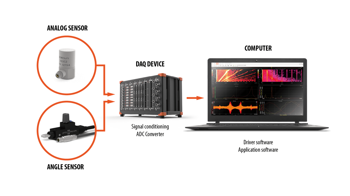
Analog sensors
First, data from one or multiple analog sensors must be acquired. Different sensor types can be used like e.g. accelerometers and microphones - to measure the sound and vibration characteristics of the Device Under Test.
More information about vibration sensors:

Angle sensors
Next to analog sensors, Order analysis requires one or multiple rotational angle sensors. The acquired angle data is used for the order tracking process performed on the analog sensor data .
Angle data indicate each time a certain fraction (or a full rotation) has occurred for the rotating component under test.
Angle sensors are e.g. encoders with a high angle resolution, or more simple tacho probes set up to measure 1 pulse/revolution - the rotational frequency.

 and angle sensors (right).")
Exceptions to required angle sensors
An exception to required angular sensors is in the cases where RPM speed data already are available and the Order Analyzer that is used supports such determined RPM signal values as data for the order tracking process.
If such RPM speed data is used for tracking, the relation to some angular sensor angle values will be missing. Therefore the order of spectral phase information will not be relative to the rotation angle. In such cases, the phase information is typically instead determined relative to the phase of the 1st. order component.
In addition to speed, RPM tracked order analysis, some analyzers also support automatic RPM tracking, also referred to as Signal Tracking or Auto Tracking. When using signal tracking, the RPM speed values needed for tracking are determined directly by signal patterns in the measured analog sensor data a(t). By this, no angular sensor or RPM signal channel is required when signal tracking is used.
When using signal tracking, note that the accuracy of the determined RPM data will be dependent on the signal-to-noise ratio of the analog sensor data that is used. In addition to that, the phase relative to the rotation angle will be missing.
DAQ device and computer
Sensors are connected to a DAQ (Data Acquisition) device which digitizes the data to be able to manipulate and analyze it on a connected computer. The computer must have Order Analysis software installed.
When the measurement system has been configured and measurements are running, the user can focus on the Order Analysis software to complete the test, analysis, and reporting tasks.
All settings defining the order analysis results are managed in the order analysis software and will be described in the sections Basic settings for Order Analysis and Additional features used with Order Analysis.
Basic settings for order analysis
In this section, parameters have been described that need to be configured in order to perform basic Order Analysis. This includes parameters used to configure the rotational angle signal, used for the order tracking process, and parameters for setting up the order spectra and extracting harmonic results.
Tracking signal setup
As mentioned in the section Order tracking theory, dynamic resampling is required to transform input time data from a discrete-time series with equally spaced samples relative to time to a discrete-time series with equally spaced samples relative to rotation angle. This is done by resampling the time data dynamically relative to an angular frequency source - the tracking signal.
Depending on the Order Analyzer one or multiple options for the tracking signal will be supported. Some analyzers might only support an analog tacho signal consisting of a series of pulses, spaced relative to the rotation angle. Other order analyzers will in addition to the analog tacho signal support digital signals e.g. a digital tacho signal and encoder signals, and will also have the option to use signals that relate to the rotational frequency (speed), like RPM channels.
If machines with high dynamic rpm, or with a high rotational vibration are analyzed (big rpm deviations during one revolution), and at the same time high orders should be extracted, then an encoder or a tacho probe with multiple pulse/rev. (180p/rev or higher) is recommended, to get higher accuracy. With more detected angular positions per revolution, the angular resolution gets higher.
Spectral settings
For different test scenarios, certain rotational speed ranges will be used for which certain amounts of relevant order components will be inspected. Depending on the test the maximum order of interest and the required order resolution will vary.
As an example, let’s consider a test of a rotating engine that varies in rotational speed between 300-3000 RPM. Order analysis of the first 20 harmonics will be performed. For the analysis, an order resolution of 1/8 order is chosen.
Line resolution
The order resolution, or more precisely the spectral line spacing, , is one of the basic customizable parameters in order analysis applications.
The line spacing depends on the data duration used for each order spectrum. To obtain a line spacing of 1/8 order, that will require the order analysis to use data of 8 cyclic revolutions for each spectrum, since:
where is the number of revolutions in each FFT Angle Block (see the section Order tracking theory).
From a time-domain perspective, this means that at 300 RPM each FFT block should have a duration of:
and at 3000 RPM the block time duration should be:
In order analyzer applications the varying time block duration is automatically handled by the order tracking process.
Number of lines
The number of lines, , indicates how many lines will be included in the produced spectra. The number of lines in a spectrum is determined by:
where is the highest order component included in the order spectrum.
Continuing our example, having a Δorder = 1/8 order, while the analysis is set to cover the first 20 harmonics, that will determine the number of spectral lines in each order spectrum be:
Required sample rate
The required sample rate of the Data Acquisition (DAQ) device depends on the highest frequency of interest for the analysis.
With order analysis, the highest frequency that will be considered is dependent on the maximum rotational speed and the highest order to analyze. Higher order and speed will require an increased sample rate.
The maximum order to analyze defines the maximum number of vibrational periods that must be detectable per cyclic revolution. In the 20th order, vibrational components will have 20 periods per revolution.
The highest frequency to analyze is also dependent on the maximum speed since that speed (RPM) determines how fast e.g. those 20 periods per rotation might happen.
First, by using the information about the maximum order and maximum speed, the highest frequency required to analyze can be determined by:
where is the highest used frequency in the analysis.
The minimum required acquisition sample rate capable of handling the analysis of up to this is at least 2 times due to the Nyquist-Shannon sampling theorem.
Typically it is recommended to use a sample rate defined as:
where factor 2.56 is used instead of 2 due to effects of the Analog-to-Digital Converter (ADC), such as aliasing effects that did not get completely removed by Anti-Aliasing Filters (AAF).
Coming back to our rotating engine example the highest frequency to analyze is:
Therefore, the acquisition sample rate should be set to:
If a sample rate is used that is lower than required, then the order spectra will not include energy components at the upper part of the speeds range and/or at the upper part of the orders range. Look at the illustration below for examples of required sample rates with respect to speed and maximum order:


Window functions
In order to reduce spectral leakage in the order spectra, a window function can be applied on the FFT angle blocks of the resampled angle domain data.
Spectral leakage is when the energy of frequency components in a signal is spread out to a broad range of spectral lines. On the contrary, of being represented by single spectral lines.
In most cases using order analysis, the rectangular window can be used since the energy content can be configured to be located mainly at distinct spectral order lines, and not in between the lines. In cases where remarkable amounts of energy are located between spectral lines, a window function should be used.
Examples of some window function shapes are illustrated in the picture below:


Reference binning setup
Reference binning covers the configuration of how order spectra can be tagged to a measured profile, like a speed or temperature profile. These settings are sometimes referred to as tag axis settings or reference profile settings.
During testing order spectra are continuously produced. Each spectrum relates to a certain period in time, a certain rotational speed interval, or to some other period of a specific reference profile.
By using Reference Binning Settings, all spectra can be collected across the measured speed range, time range, or another measured range producing 3D spectra. It is additionally referred to as spectrograms or waterfall plots. An example is illustrated below.


A couple of reference profiles are described below, presenting some examples of what order spectra could be correlated with. Reference binning settings can often be adjusted in post-processing or Analyze mode as long as the measured time data has been stored.
Rotational speed reference
Analyzing order spectra with respect to measured rotational speed is widely used in various application domains. This is because speed variations will affect the rotating test object to pass through all sorts of noise and vibrational phenomena revealing e.g. critical speeds at structural resonances.


G-force reference
Other reference quantities than just time and rotational speed can also be relevant to correlate with spectral data, to investigate how different quantities are linked to spectral energy patterns.
For example, during the take-off and landing of aircraft or when aircraft do manoeuvres in the air, the g-forces can impact the engines to have increased vibration and deflection levels for certain rotational components. Such as the inner and outer fan blades of gas turbine engines.


Temperature reference
Temperature is another quantity that might be of interest when analyzing order spectra of measured noise and vibration data. Correlating spectral data to a temperature profile of a measured engine can provide insight into how well the engine is performing across a temperature range.
Wind speed reference
Wind speed is an important quantity to measure while acquiring data from wind turbines. Wind turbines experience changing wind speeds and the rapid wind blows which cause rotational speed variations. The speed variations make order analysis an obvious choice to use when inspecting spectral energy components.
By using the wind speed as a reference profile for the order spectra, investigations can be performed revealing how different wind speeds affect the spectral energy patterns of measured noise and vibration.
For some order analyzer applications, the reference binning settings are handled in the graph displays only while in other applications the binning settings are part of the analysis setup. Having the binning settings included in the order analysis setup enables the waterfall data to be stored and exported as separate data channels.
Bin width
Order analysis applications will typically include parameters for determining how the spectra will be collected over a selected reference profile.
For example, the binning width determines the resolution on the reference axis. As illustrated in the previous spectrogram, the binning width or delta width (REF) determines the range for which all spectra should be collected to the same reference bin. By selecting a narrow bin width spectra will be separated into more bins than if a broader bin width is selected.
The bin width should be set small enough to allow for proper detection of e.g. critical speeds on a speed profile.
For analysis of fast run-up or coast-down testing, the rate of produced spectra must also be fast in order to obtain spectral data in all the reference bins.
A fast rate of produced order spectra can be achieved by increasing the order Line spacing (as described in the section Line resolution). Since such a lower line resolution will shorten the FFT Angle Block duration, the rate of produced spectra will increase.
Bin direction
Some order analysis applications include a parameter determining in which test Directions the spectra will be collected. Having e.g. a speed profile as a reference, the direction parameter can be set to only collect run-up spectra (when the RPM is increasing) or only coastdown spectra (when the RPM is decreasing) or to collect spectra in both directions.
Bin hysteresis
Bin hysteresis is used to determine when order spectra will be assigned to the next bin.
By setting a higher hysteresis value the reference profile has to vary more before the order spectra are assigned to other bins. This parameter can be adjusted to keep a steady binning of spectra even though the related reference profile contains many smaller variations, e.g. small speed variations in an unsteady engine.
Bin update criteria
The bin update criteria determine how collected spectra in individual bins are processed. Some typical options are to either average together all spectra collected in each bin, or to only keep the newest spectrum in each bin. Another option is to set the bin update criteria to keep the maximum order lines across all spectra in each bin. This option can be used to indicate worst-case scenarios.
Harmonic extraction settings
Harmonic order values can usually be extracted from the produced order spectra across the test time duration or across the measured range of a reference channel.
Each extracted harmonic will produce one value per produced order spectrum.
As mentioned in the section Extracted harmonic orders, this can be very useful when knowing which harmonic components are important to inspect. Extracted harmonics can also simplify the configuration of automated detection systems that must trigger an event if some rotational-related misbehaviour arises.
Extracted orders can be either integer order numbers or fractional orders such as sub-harmonics or half-integer orders. Which harmonics to extract depends on the test application and expected sources of rotational problems, (see the section Detecting sources of vibration).
An illustration of extracted harmonics over time and over a speed range is shown below.


n the illustration above, the first harmonic shows higher values as the speed increases which might indicate present unbalance. The 2nd harmonic does not indicate critical values. However, the 10th harmonic has high values at certain speeds which could relate to a critical frequency.
Additional features used with order analysis
Markers, tolerance curves, and alarm events
During order analysis it can be beneficial to have access to certain marker types for the graph displays, providing quick ways to extract specific information from the data results.
Common marker types used with order analysis is e.g.
Free markers - determine the value and axis position of a user-defined data point.
RMS markers - calculating the total RMS value over a user-defined order range.
Max markers - determine the user-defined number of max. values and their axis positions.
Harmonic markers - determine user-defined numbers of harmonic component values.
Trigger marker - triggering an event when a user-defined value is exceeded.
Vector cut markers - extract a user-defined order component across the measured reference bin range or a specific reference bin across the analyzed order range.
Some order analyzer applications support the ability to produce derived channels for each added marker, which outputs values each time the related graph data is updated.
Processing markers manualSoftware user manual for DewesoftX processing markers.
An example of using markers is illustrated below, where a Max. marker is set to highlight the 5 greatest data points (highest peaks) and to list the values and axis positions in a marker table:


When performing order analysis on operating machinery for monitoring purposes, tolerance curves and alarm detection can be valuable tools. This is for pointing out time for maintenance, or to take action quickly in cases of rotating element failures.
If tolerance curves are supported in the order analysis application, the user can define data points that create lower and upper range limits for accepted order values. If a certain order component e.g. exceeds the upper tolerance limit value defined at that order position, then an event is triggered. The triggered events can be configured to start a series of user-defined actions, such as:
Start recording data (e.g. with negative delay applied, to include the instance of the trigger event).
Print a report with event-related data results.
Output a digital trigger signal to 3rd. party hardware, that will handle additional actions.
Send an email with relevant information about the trigger event.
An example of an ordered spectrum with a defined upper tolerance curve is illustrated below:

 for an order spectrum (blue), relating to a certain speed RPM width.")
Weighting and scaling
Order analysis applications can support different types of data manipulations in order to obtain results that relate more directly to what is relevant to the inspection.
Amplitude scaling
Amplitude scaling determines how the amplitudes of the spectral lines get scaled.
Based on the specific signal type, and the type of measurement performed, certain scaling formats will be more convenient and better used.
Normally, the relationships among scaling formats in order analyzers are based on the assumption that spectral lines represent individual sinusoids. Therefore, the following relationships hold:
Peak (pk) is the signal-positive peak amplitude.
RMS (RMS - Root Mean Square) is the signal RMS amplitude. For sinusoids, RMS relates to the peak value by:
Peak-to-peak (pkpk) is the signal minimum-to-maximum peak amplitude. For sinusoids, pkpk relates to the peak value by:
Acoustic weighting
Acoustic weighting functions are used for sound pressure signals. When analyzing sound and noise signals acoustic weighting filters can be applied in order to take audible human perception into consideration. Humans do not perceive all frequency components to be equally loud, even though they have the same sound pressure level. Acoustic filters are defined to take that sound perception into account.


Differentiation/Integration
Differentiation/Integration functions are used mainly for vibration signals to change the physical quantity. A typical scenario for this is when transforming data from the acceleration domain to the displacement domain. Changing the physical quantity to displacement from acceleration can be helpful when using acceleration sensors, and you want to inspect spectral or harmonic displacement values. E.g. for monitoring extracted 1st-order displacement values of a turbine engine, based on acceleration sensor measurements.


Order tracking filters
In some cases, it can be relevant to perform additional types of analysis on certain order components of measured time signals. For example, when performing sound measurements of a rotating machine, it might be of interest to playback and hear the sound from only certain harmonic components. Hereby the sound from different rotational components can be investigated and optimized in order to obtain a better overall sound quality and sound experience of the machine.
By using the order tracking filters such specific order components can be extracted, filtering out all other components. Such types of filters are different from many other types of filters. This is because the tracking filters follow/track the rotational speed, and dynamically shift the band-pass filter centre frequency up and down based on the current measured speed.
Gathering a collection of derived signals from different components that all relate to different harmonic components, gives the ability to quickly overview the influence on the overall system when modifying specific components. For example, analyzing the influence of exchanging a certain rotational component in a car can be done by exchanging the related order components in the overall signal.
Additional applications using the order tracking
Next to order analysis, the fundamental tracking mechanism is also used in other applications as well. Some of these additional applications will be described shortly below.
Orbit analysis
In addition to real-time Order analysis, Orbit analysis is a widely used application for inspecting rotor and shaft movement in rotating machinery.
Orbit analysis uses pairs of proximity probes together with angle sensors in order to determine the shaft movement and positioning under operation.
Like order analysis, orbit analysis transforms the time data into the angle domain, by order tracking, in order to get the required shaft movement in relation to the angular position.
Learn more:


 shows the shaft centerline XY position over a speed range. The polar plots (right) show the 1st order displacement of the two proximity probe locations together with the phase relative to the key phasor position of the angular sensor, over a speed range.")
Non-stationary ODS
Some software applications support structural analysis insight based on non-stationary ODS (Operational Deflection Shape). This is also referred to as run-up coastdown ODS and is spectral ODS analysis, but performed in the order domain. For non-stationary ODS, order tracking is again used to handle speed variations during machine operation. The order ODS results can determine structural deflections over the measured order range, and the deflections can be animated on a structural geometry.
Tracked envelope analysis
In theory order analysis can also be performed on enveloped (amplitude-demodulated) time data.
Envelope analysis is a tool that can be used to inspect e.g. wear of gears and bearings by focusing the analysis on transient energy components found in the higher frequency area. Increasing amplitude values at such higher frequencies can indicate the non-ideal operation of rotational components.
By using envelope analysis the amplitude and rate of such high-frequency transients are analyzed to determine which rotational component is the source for those energy components, as well as to determine its health state.
If order analysis is performed on enveloped time signals the rate of these transient components will be specified at spectral lines in the envelope order spectra. This is beneficial if the measurements relate to varying speeds.
References
1. Dewesoft
Measuring RPM, Angle, and Speed Using Digital, Encoder, and Counter Sensors
FFT Analysis (Fast Fourier Transform): The Ultimate Guide to Frequency Analysis
2. Data physics
Order Analysis, Order Tracking, and Filtered Orders
3. Others
4. Brüel & Kjær
Application Note: Time Domain Averaging Combined with Order Tracking, by N. Johan Wismer
5. Crystal Instruments
An Ear for Gears - Understanding Gearbox Signatures
6. Power-MI, Eccentricity