


What is Modal Analysis: The Ultimate Guide

March 15, 2021
In this article, you will learn about structural dynamics, modal testing, and modal analysis with enough detail that you will:
Understand what modal analysis is and what is it used for
Learn how modal analysis is performed
See how modal analysis works
The most important elements of a typical modal analysis survey will be presented in the same order that they are normally performed, as outlined by the table of contents.
Introduction to modal analysis
What is modal analysis?
Modal analysis is an indispensable tool in understanding the structural dynamics of objects - how structures and objects vibrate and how resistant they are to applied forces. The modal analysis allows machines and structures to be tested, optimized, and validated.
Modal analysis is widely accepted in a broad range of applications in the automotive, civil engineering, aerospace, power generation, and musical instruments industries, among countless others.
Natural resonance frequencies of the objects and damping parameters can be calculated, and mode shapes can be visualized on an animated geometry of the measured objects.
The collection of modal parameters - natural frequencies, damping, and mode shapes - is referred to as a Modal Model.
To determine accurate modal models thorough modal analysis must be performed based on accurate modal test measurements.
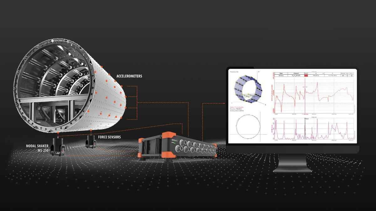
Modal Test and Analysis typically involves:
One or more exciters, such as modal shakers or an impact hammer
Force transducers that acquire the input excitation signals
Accelerometers that acquire the output response signals
A DAQ device (Data Acquisition) device to display and record the test
A computer with a Modal Test and Analysis software application


Learn more:

What is a modal analysis used for?
Modal analysis is heavily used to analyze and validate designs like aircraft frame parts, wind- or gas turbine blades, vehicle chassis, and any critical structure that is exposed to forces that might induce harmful or even destructive resonant frequencies without damping.
At resonance frequencies with critically low damping, an object can react/vibrate strongly from even small amounts of input force or energy.
Modal Analysis can give the user an overview of the object's natural frequencies, damping parameters, and structural mode shapes.
This knowledge allows engineers to modify and optimize the object’s design to be less sensitive to applied forces.
It is also used to correlate Finite Element analytical models with real-life prototypes by using the damping characteristics, discovered by empirical testing.
Design optimization is often used to fulfill today's fuel economy demands and the inherent push for lighter structures. Structural Dynamic Analysis is mandatory in many cases, to learn how the structure reacts to a given optimization.

 of a plate geometry at different resonating frequencies")
How is a modal analysis performed?
To ensure high-quality results a modal survey involves these key elements:
Modal test
Preparations
Equipment
Preliminary Tests
Geometry
DOFs
Excitation technique
Configuration
Measurements
FRF
ODS
Validation
Coherence
Modal analysis
Parameter identification
MIF
Curve Fitting
Mode Selection
Stability Diagram
Natural Frequencies
Damping
Mode Shapes
Modal model validation
AutoMAC and CrossMAC
Mode Shape Scaling
Synthesis
Modal analysis can be based on structural test measurement or simulated FEM models, (Finite Element Models). This article will mainly focus on modal analysis based on real modal test results. Correlation Analysis between simulated Finite Element Analysis (FEA) models and test empirical test results will be covered in another article.
Modal testing
What is modal testing?
Modal testing and the acquired test data are the basis for performing modal analysis and making conclusions on the structural dynamics of test objects.
This section will cover enough information to get a basic understanding of modal testing and how to acquire data for the subsequent modal analysis.
Modal Testing can be performed with either applied artificial excitation sources, to get the test object to vibrate, or by having the test object running under operational conditions, in-situ testing, where in-situ vibrations will be present.
Learn more:
Experimental modal analysis (EMA)
Experimental Modal Analysis (EMA) tests can be performed both in the field and in more controlled lab environments. Testing in the lab has the advantage of a higher signal-to-noise ratio (SNR) and the ability to easily change the test setup.
When doing EMA testing, objects are excited by artificial forces and both the inputs (excitation) signals and outputs (responses) signals are measured and used to estimate Modal Models.
Operating deflection shapes (ODS)
Operating Deflection Shapes (ODS) is a simple way to do dynamic analysis and see how a machine or a structure moves within its operational conditions. ODS tests have no applied artificial forces and only response vibration signals are measured.
A modal model can not be estimated from ODS measurements but it provides structural deflection shapes which improves the structural analysis of operational DUTs.
ODS is used successfully for machine conditioning monitoring and in civil engineering applications e.g. on bridges, buildings, and other structures that are difficult to excite with artificial forces.
Operational modal analysis (OMA)
The modal test measurement procedure for Operational Modal Analysis (OMA) is similar to ODS, but their analysis part is different. How ODS and OMA differ is explained in detail in the section ODS vs OMA described.
Test preparation
Before starting a modal test some test preparation is required, including:
Mounting of the Test Structure
Type of excitation force(s)
Location(s) of excitation (driving points)
Hardware and sensors to measure the force(s) and responses
Geometry Model
Mounting of the test structure
When performing modal testing the DUT (Device Under Test) must be able to vibrate dynamically in ways that will reveal all and correct natural frequencies and mode shapes of the structure.
To pursue free vibration patterns, or similar vibration patterns as expected when the structure is operating in real life, materials like rubber bands, elastic wires, foam pads, and other materials providing a soft elastic system are often used to hang or place the structure on at the locations the structure is designed to be fixed.
If e.g. the test structure is fixated at some positions under test, that is going to vibrate freely when the test structure is operating in real life, then the measured dynamic properties will not fully relate to the real-life usage of the structure - since adding stiffness to the structure will shift the frequencies upwards, and it might also cause some mode shapes to be undetected.
Rigid body motion
Rigid motion, or rigid body modes, are vibrations of the whole DUT as a rigid object and do not provide information on the structural dynamic properties of the DUT (the flexible modes). Such rigid body modes are related to the selected support configuration.
Depending on how the DUT is mounted the rigid body modes might affect the flexible modes of the structure in an unacceptable manner. The impact of the rigid modes on the flexible modes depends on how close in frequency the rigid modes are to some flexible modes, and on what is determined to be an acceptable accuracy of the measurements.
A rule of thumb is often to accept the modal data if the FRFs show greater than a 10:1 frequency ratio between the rigid body modes and the flexible modes, e.g. last rigid mode at 1 Hz and first flexible mode at 10 Hz. But, again this will always depend on the agreed accuracy of the specific application since some flexible modes will be affected to some extent.
If a different support configuration is introduced then the best practice is to make an evaluation of how this affects the flexible modes.
Types of excitation force(s)
Different input excitation types can be selected for EMA testing. Which type to choose depends on the user scenario. For example:
Impact excitation with a modal hammer is often the best solution for smaller homogeneous structures and for field measurements since it is fast, portable, and requires no fixturing.
Sine sweeps, random noise, and other excitation types from a modal shaker/exciter are often the best solution for larger complex structures, where more in-depth analysis is required, including non-linearity studies, low Crest Factor, and high Signal/Noise ratio.
For complex structures, multiple shakers might be required if no excitation locations (reference DOFs) can be found where all the modes have sufficiently high participation for proper modal model extraction. Furthermore, with modal shakers, the force level can be precisely controlled.
In some other scenarios, non-standard exciters are chosen, such as e.g. electro-hydraulic shakers and drop hammers, together with other excitation methods that provide better input excitations for some special purposes.
Location of excitation (driving points)
For EMA testing it is important to excite the object at location(s) that will reveal most of its vibrational characteristics. For example, if an object is excited at a location where some vibration mode patterns always have minimum vibration amplitude, then these modes will not absorb energy and be excited.


To identify proper excitation locations, pre-testing is often performed where different driving point locations are compared. If a Finite Element Model (FEM) is available this can also be used to determine good excitation locations.
Because ODS and OMA testing, do not use input force signals, it is especially important to select reference response DOFs that aren’t in a nodal position of any mode, such that they include energy components from all the structural modes.
Hardware and sensors to measure forces and responses
For EMA testing, input excitations are usually measured by force transducers or impedance heads at the driving points. An impedance head includes both a force sensor and an accelerometer and is often used to obtain driving point measurements.
As an alternative to impedance heads, an accelerometer can be placed close to the force sensor at the excitation points. Response signals are very often measured with accelerometers, but other probes can also be used.
Multiple accelerometers are often chosen to optimize data consistency and reduce measurement time, and for larger complex structures the number of accelerometers can easily get large.
If the number of response sensors is limited then "roving" measurement can be used. In this scenario, a group of response sensors is moved around between test runs. These sub-tests add up to a full measurement of all DOF locations.
In the cases where different modes deflect in different orthogonal directions, triaxial accelerometers can be used, since they contain three sensors oriented in an X Y Z pattern.

 Impedance head - PCB type 288D01 (Middle) Force sensor - PCB type 208C03 (Right) Accelerometer - PCB type T333B32")
Sensors are available with different sensitivities and thus different frequency ranges. Select the sensors such that they support the frequency range and level range included in the modal test. These dynamic ranges must also be supported by the chosen DAQ device.
The weight of the sensors is also important to take into account since the object will vibrate differently when the Mass Loading from sensors is relatively high. A rule of thumb is that the sensor's mass should be less than 1/10 of the object’s mass.
Check out Dewesoft's modern, high-quality digital data acquisition systems


Learn more:

Geometry model
In most cases, a geometry model should be created before starting a modal test.
The geometry is built-up by points, trace lines, and surfaces, where some of the points indicate the locations to measure - also called DOFs (Degrees Of Freedom). DOFs define the node point locations and directions to measure, for example, ‘0012, Z+’.
Geometry models help engineers select the best set of DOFs to measure, overview and guide the measurement process, and visualize the determined mode shape deflections of the test object.


How to perform a modal test?
When the test preparations are done the actual modal test can begin. For EMA testing, depending on the test situation it might be better to use one or multiple modal exciters and one or multiple response sensors. These different test configurations are grouped into the sections ‘Single-reference Modal Tests’ and ‘Multi-reference Modal Tests’. Hereafter a section will describe ODS Testing.
Single reference modal test
In some test cases, it is sufficient to extract the modal model from measurement data with only one reference DOF.
The assumption is that the selected reference DOF contains information about all the modes. This is possible if the reference DOF location can be chosen such that none of the modes is in a nodal position. In practice, this means that all the modes should be sufficiently "present" in the measured data.
Single reference roving hammer test
For a Roving Hammer Test, this means that only one response DOF is needed, i.e., only one accelerometer position. For such a roving hammer test the accelerometer response DOF will be used as the reference DOF, while the hammer will rove between the DOFs. This is an example of what is called a Single-Input Single-Output (SISO) test configuration.


Single reference roving accelerometer(s) test
Another type of roving test can also be selected, where it is the modal exciter (e.g. hammer or shaker) which is used as the reference DOF, while one or a group of accelerometers will rove until all DOFs have been measured. This is also referred to as a Roving Response Test.
If multiple accelerometers are used it will be referred to as a Single-Input Multiple-Output (SIMO) test configuration.

The disadvantage of this configuration is that the mass of the accelerometer affects the structure differently at every point, and therefore influences the measurement. This effect is called Mass Loading.
Also between each roving measurement, the sensor has to be moved and mounted again, which is more time-consuming than a roving hammer test.
Single reference shaker test
For a single reference modal test (where it is sufficient to extract the modal model using only one reference DOF) a modal shaker can also be used.
A modal shaker is often chosen for modal tests requiring a more accurate modal model determination.
When using a modal shaker, the reference DOF is very often chosen to be the shaker excitation location, e.g. since it normally is more time-consuming to relocate (rove) the shaker than roving a group of accelerometers.

Multi-reference modal tests
Some test cases require measurements with more than one reference DOF. This is the situation when it is not possible to find a proper reference DOF where all the modes are sufficiently "present" in the measured data.
For example, structures may exhibit different modes with predominant modal deflections at different parts of the structure. Such modes are often referred to as local modes.
An example of this is complex structures composed of several different parts with different structural properties.
Multi-reference testing is also required in cases where the test object has more modes with the same resonance frequency. This is often referred to as "repeated roots" and closely coupled modes.
An example of repeated roots is when having certain symmetrical structures. In such cases e.g. two bending modes perpendicular to each other could be closely coupled regarding their resonance frequency.


The number of reference DOFs measured must be (at least) equal to the number of modes at the same frequency.
Multi-reference roving hammer test
Regarding hammer testing, including multiple reference DOFs in a modal test, can be achieved by using multiple response sensors as reference DOFs.

Multi-reference shaker test
Multi-shaker tests are normally performed with more accelerometer sensors - hereby having a Multiple-Input Multiple-Output (MIMO) configuration.
The main advantage of using multiple shakers is that the input-force energy is distributed over more locations on the structure. This provides a more uniform vibration response over the structure, especially in cases of large and complex structures and structures with heavy damping.
To get sufficient vibration energy into these types of structures, the input excitation level is sometimes set too high when only a single shaker is used. This can cause non-linear effects and give bad estimations of the modal model. Excitation in more locations often also provides a better representation of the excitation forces that the structure experiences during real-life operation.
Using multiple shakers instead of roving a single shaker also has the advantage of providing more consistent data and reduced measurement time. Consistent data is crucial for the modal analysis performed on multi-reference modal test data.
When using multiple modal shakers, the excitation sensors are used as reference DOFs.

Distinguishable modes at reference DOFs
In multi-reference configurations, the mode shapes that are to be extracted have to "ook differently" at the reference DOFs. In other words, the mode shapes for these modes must be linearly independent at the reference DOFs. This is achieved by selecting proper DOFs as reference DOFs.
As an example, a plate might have two closely coupled modes (resonance around the same frequency), wherein the deflection is similar for both modes at certain DOFs. Imagine that two reference DOFs are placed at two similar deflecting DOFs. In this case, the measured reference DOF data will not include information needed to separate the modes.
, first torsional mode (middle), and both modes together with a good and a bad position for two reference DOFs (right). If the modes have repeated roots, then the reference DOFs must be selected such that the modes reveal their differences.")
Multi-reference excitation types
In multi-reference shaker tests, uncorrelated random excitation signal types are normally used. The random excitation types can be continuous, burst, or periodic random.
Sinusoidal excitation signals can also be used to perform Sine Testing, e.g. Stepped Sine testing or Normal Mode Tuning.
With Sine Testing it is possible to control the excitation force level, for a particular frequency, at the individual excitation DOFs, together with the phase pattern between them.
With the ability to control the excitation levels and phase pattern at DOFs, it is possible "to tune in" to a specific mode (Normal Mode Tuning). This can be very useful when a detailed investigation of single modes is desired, e.g. when performing a non-linear investigation for specific modes.
With sine testing, all applied energy can be focused on exciting one specific mode at a time. In this way, a significant amount of the input energy can be reduced or focused at one frequency. Compare this to random excitation signals, where the energy is distributed over the full frequency span, covering all modes simultaneously.
ODS (operational deflection shapes) testing
ODS (Operational Deflection Shape) Testing can be a valuable tool for analyzing and determining modifications for dominating structural vibrations on operating structures, where normal EMA is difficult to perform.
Examples of operational test conditions can be continuous signals from a running engine, or transient signals from earthquakes, explosions, drop-tests, and many more.
ODS testing determines the structural deflection shapes of an operating DUT by measuring the amplitude and phase information of the DOFs.
ODS Testing does not use input excitation signals, but only output response signals. One or more of the response DOFs are selected as the reference DOF(s) to extract the phase information.
Note that the selected reference(s) need to cover energy from all frequencies/orders of interest.
The deflection shapes can be determined by either Time ODS, Spectral ODS, or Non-stationary ODS (used for varying speed testing). In all cases, the ODS results are animated deflection shapes on the Geometry and the related amplitude and phase information.
Time ODS
Time ODS results express the overall deflections of the operating DUT, where the user can adjust the time for where to look at the deflections.
Time ODS testing uses the measured time signals of the DOFs to extract the amplitude levels and the phase related to the reference DOF(s). This is done for all points in time, and the deflections can hereby be animated over a time axis.
Note that since Time ODS testing uses the time signals to extract the phase information, it is difficult to use when performing roving accelerometer testing. In these cases, accurate triggering mechanisms are required to ensure that all roving sets of measurements are aligned with respect to phase. Normally Time ODS is performed when enough accelerometers are available to cover the DUT without roving.
Spectral ODS
Spectral ODS results express the deflections of the DUT at individual frequencies determined by the user.
Spectral ODS testing uses the processed frequency data of the DOFs to extract the amplitude and the phase related to the reference DOF(s). This is done for all frequency components in the spectral data, and the deflection shapes can hereby be animated over a frequency axis.
Non-stationary ODS
Non-stationary ODS results normally express the deflections of the DUT at individual orders of rotation, determined by the user.
Non-stationary ODS testing normally uses dynamic resampled (Order Tracked) spectral data of the DOFs to extract the amplitude and the phase related to the reference DOF(s). This is done for all order components in the rotation-related spectral data, and the deflections can be animated over an order axis.
Learn more:

Rotating components like gears and bearings of the DUT often rotate at different orders or fractions of the measured speeds(s). These parts will be indicated as different-order components that are independent of the speed. Hereby deflection shapes can be focused on different rotating DUT components, by looking at the different orders.
If the shape deflections at a specific order change with speed variations then it indicates that the related DUT component is affected by such speed variations.
Averaging of test measurements
It is important to average multiple measurements taken at the same DOF locations.
Why? Each measurement includes some random noise that can affect the determination of the resonance frequencies of the system and mode shapes. By averaging multiple measurements, the random noise components can be reduced.
A random noise will be reduced more if a higher number of averages are chosen, and it is up to the engineer to decide a preferable number of measurement blocks to average. This decision is a balance between the desired quality of the results and the required test time.
In general, a rule of thumb is to average across:
32 to 64 averages for shaker testing, and
4 to 8 averages for hammer impact testing.
Normally Modal Test application software lets the user specify the number of averages to use at each DOF measurement. For normal impact excitation testing (with one impact per measurement block), this means that the user should impact the set of DOFs locations each equal to the number of averages specified.
Looking at Coherence functions is a primary validation tool when performing Modal Testing, but don’t be misled by a coherence value of 1 after a single measurement has been taken.
By definition, the coherence function is based on multiple measurements and therefore only provides useful data after averaging has been performed.
Averaging should be done on the data for the individual DOF locations and not across all DOFs.
For example, it is valid when averaging the Autospectra and , and the Cross-spectra based on the same DOFs. Modal Tests results like FRFs and Coherence functions are when calculated based on those averaged spectra. Autospectra and Cross-spectra are described more in (Appendix).
What is a modal hammer?
A Modal Hammer is used for hammer impact tests, and is typically carried out on a simple structure or is used as a quick survey before the more complex modal shaker test. It involves relatively less equipment, namely a sensor without the attachment of the shaker to the structure. In general, it takes little time to set up and carry out the modal test where a smaller amount of measurement points are sufficient.


Types of modal hammers
Modal hammers have different sizes and specifications depending on the types of structures they are designed to excite.

 Brüel & Kjær Modal Sledge Hammer - Type 8210 (right)")
To get an overview of which modal hammer is best suited for a certain job, the table below can be used as a guideline.
| Hammer Size | Applications | Range Scale | Sensitivity | Mass |
|---|---|---|---|---|
| Small | Small Structures:Circuit Boards, processors & memory modules, and other delicate articles. | < 100 lbf pk, < 444 N pk | > 50 mV / lbf, >11.2 mV / N | < 0.36 lb, < 0.16 kg |
| Medium | Medium Structures:car frames, engine blocks, small electric motors, and other medium-heavy devices. | 100 - 1.00k lbf, pk, 444 - 4.44k N pk | 50 - 5 mV / lbf, 11.2 - 1.10 mV / N | 0.36 - 1.00 lb, 0.16 - 0.45 kg |
| Large | Heavy Structures:Pumps, compressors, weldments, impellers, building foundations, and other very large structures. | > 1.00k lbf, pk, > 4.44k N pk | < 5 mV / lbf, <1.10 mV / N | > 1.00 lb, > 0.45 kg |
When the optimal hammer has been selected, additional properties should be considered:
Frequency response - frequency range, selecting optimal impact tip to use
Hammer dimension and weight - practical considerations
Measurement range - providing sufficient impact force level
Sensitivity - finding a balance between too-weak signal levels and overloaded levels.
Non-linearity - consistency, and accuracy
Hammer tip
Regarding the frequency range to include in the modal test, then selecting the correct hammer tip is important. A harder tip material provides a larger frequency range, but it can also make it more difficult to avoid double hits. A softer hammer tip gives a longer impact time which will give a better energy transfer to the structure at lower frequencies, but the frequency span in the modal test will be smaller.
As a rule of thumb choose a hammer tip material with a frequency response where the attenuation is less than 6 dB at the upper frequency of the modal test.


What is a modal shaker?
Modal shakers are vibration shakers used to excite large or complex structures and to achieve high-quality modal data. In comparison to modal hammers, modal shakers have the ability to excite the structure in a broader frequency range, and with many different signal types, best suited for different structures and ideal for accurate test results.
Also, modal shakers can be controlled to excite the structures with certain user-defined excitation levels, which can be used to gain a flat or shaped excitation curve with reference to the excitation frequencies. By controlling the shaker excitation level the structure can be protected from critically high amplitude deflections, and different levels can be tested to analyze non-linear effects.
Multiple shakers can be used together with and without controlled amplitude and/or phase patterns. Using multiple shakers on complex structures gives a more realistic force excitation and better investigation of all mode shapes.
Types of vibration shakers for modal testing
Various types of shakers can be used as modal shakers:
Permanent Magnet Shakers
Modal Shakers
Inertial Shakers
Each type has its advantages and disadvantages. For example, regarding the maximum excitation force level, the frequency range, and not least, the way that the shaker is mounted to the DUT.
Permanent magnet shakers
Permanent Magnet shakers are general-purpose types that allow the DUT to be fixed directly to the shaker armature, and the vibrating surface area can be enlarged by using a head expander to accommodate larger objects.
Permanent magnet shakers are typically used for:
Vibration testing of micro parts, and modal testing of assemblies and electronics
Shock Testing
Sensor Calibration
Fatigue and Resonance Testing
Education and Research
Modal shakers
A Modal Shaker (aka "Modal Exciter") offer some advantages over normal vibration shakers when performing modal testing.
For instance, instead of fixing the DUT to the shaker armature, a modal shaker is attached to the DUT via a connection rod called a "stinger."
Modal shakers are designed with a through-hole armature for the stinger, such that the stinger can be adjusted with the required length to the DUT without moving the shaker, which simplifies the setup.
Modal shakers are typically used for:
Electronic circuit boards
Subcomponents
Machinery
Vehicles
Aircraft and other large structures

Modal shakers are available with a range of specifications, as shown in the table below:
| Output Force | Frequency Range | Displacement PkPk |
|---|---|---|
| ~ 20 N, 4.5 lbf - 500 N, 112 lbf | ~ 0 Hz - 12 kHz | ~ 5mm, 0.2 inch - 25 mm, 1 inch |
The stinger is a thin flexible rod that improves the accuracy of the modal test by mainly transmitting force in the axial direction to the force sensor or impedance head. The lateral flexibility also protects both the DUT and the modal shaker from critical forces.


Inertial shakers
Inertial shakers are used for structures requiring excitation in lower frequency bands. These shakers are directly connected to the structure, and the inertia motion of the shaker mass provides the necessary forces to the structure.
Inertial shakers are well-suited primarily for the same application as modal shakers: modal testing as well as a variety of general vibration testing applications. Depending on the dimensions of the structure and the desired excitation frequencies and levels required, either modal shakers or inertial shakers can be used.


Inertial shakers are available with a range of specifications, as shown in the table below:
| Output Force | Frequency Range | Total Shaker Mass |
|---|---|---|
| ~ 5 N, 1.1 lbf - 40 N, 9 lbf | ~ 10 Hz - 3 kHz | ~ 0.05 kg 0.11 lb - 0.5 kg, 1.1 lb |
Learn more:

Shaker excitation signals
We know several types of vibration shaker excitation signals:
Random
Burst Random
Pseudo Random
Periodic Random
Sinusoidal Chirp
Swept Sine and Stepped Sine
Let's look at each type in detail.
Random
Random (or Pure Random) excitation provides “white noise” with random variation of the amplitude and phase, over a defined frequency range. With random excitation, there will be a leakage in the spectral estimates, since the random signal is not periodic. Leakage can be handled to some extent by using a time weighting window (such as Hanning window), and by increasing the spectral resolution, (decreasing the spectral line spacing ).
Random excitation provides a pretty good Crest Factor (the peak to RMS ratio) and Signal to Noise ratio. It is one of the best signal types to use (while averaging), for the linear approximation of a system in case of non-linearities. The required averaging will increase the test time.


Burst random
Compared to Pure Random excitation signals, Burst random, on the other hand, can be leakage-free with the right burst rate selected. If this is the case, a uniform window (no window) can be used. The burst random excitation type is a relatively fast signal type to use, but the Crest Factor is increased and the signal-to-noise ratio is reduced compared to Pure Random excitation.


Pseudo random
The pseudo-random excitation type is fast, leakage free and provides a pretty good Crest Factor and signal-to-noise ratio. On the other hand, a pseudo-random signal cannot be used for linear approximation of a nonlinear system.
With pseudo-random excitation signals, the same block of random time signal is repeated, running in a loop. Hereby the test structure will settle its vibrations to a periodic response, by which leakage-free measurements can be achieved, by using a rectangular weighting window.


Pseudo-random signals are ergodic stationary signals chosen to have a repeating time block length equal to the used FFT time block length ( ) and to only consist of energy content at integer multiples of the FFT frequency lines ( ).
For pseudo-random signals, the energy at the spectral components is fixed, but they have random phases. The fixed energy content at the spectral components can be Constant over the used frequency range or Shaped to concentrate energy around resonance frequencies.
Periodic random
Periodic Random signals are a combination of random and pseudo-random signals, which provide leakage-free measurements and the best linear approximation of a system. However, the test time is longer than then using random or Pseudo-Random excitation signals.
A periodic-random signal is a pseudo-random signal which changes over time. For example, when a pseudo-random signal has been running for some number of FFT time blocks ( ), it changes to a different pseudo-random signal. This process will continue through the modal measurements.
Using this method, the structure has time to settle in on the steady-state responses given by the different pseudo-random signals. Only the last time block for each pseudo-random signal (when the structure is settled) is used for the modal analysis.


Like Pseudo-Random signals, Periodic Random signals are ergodic, stationary random signals. They consist of energy only at integer multiples of the FFT frequency increment. However, with Periodic Random signals, the spectral content has both a random amplitude and a random phase distribution.
Sinusoidal chirp
With a chirp signal, a sinusoidal sweep runs through a defined frequency range for every FFT Time block T. Chirp signals are in the same category as pseudo-random signals, having the same useful characteristics and disadvantages. But, for sinusoidal Chirps the Crest Factor is reduced to less than 2, the signal-to-noise ratio is high and the spectral content has a flat magnitude and a smooth phase. Chirp signals are well-suited for the measurement of nonlinearities in structures.


Swept sine and stepped sine
Swept Sine and Stepped Sine have the same signal characteristics as Chirp, but the full frequency range is not covered in each FFT time block ( ). Instead only a smaller part of the frequency range is processed together, and the final full-range measurements are built up of a series of processed frequency components.


Like Chirps excitation, Swept Sine and Stepped Sine are good to use for examining nonlinearities in structures, and with the user-defined sweep or step rates it is possible to analyze certain frequencies and modes easily and in more detail.
With stepped sine, the structure gets time to settle into a steady-state response before any data is extracted for that frequency. After the extraction, the signal steps to the next frequency, and the structure settles again. This process continues through the full frequency range.
At different step frequencies, the amplitude can be controlled. If multiple modal shakers (and therefore multiple excitation signals) are used simultaneously, then their phase pattern will also be controlled.
In many software applications, dynamic resampling is used for Swept Sine and Stepped Sine, where the FFT time block has a dynamic time length depending on the sinusoidal frequency. Instead of fixed ( ), a dynamic time equal to a number of sine periods is defined to be the FFT time block size.
Modal tests results
FRF (frequency response function)
The primary result to extract from Experimental Modal Tests is the Frequency Response Functions (FRFs) between the reference DOFs and all DOFs on the geometry.
FRFs are measures of the relation between output response motion and the input excitation force, and hereby indicate the inherent properties of a linear system.
FRF values are calculated for each FFT frequency component, providing FRF functions over the measured frequency range.


The magnitude of an FRF is often in units [ ] or [ ]. At frequencies with high FRF magnitude values, the structure is more sensitive and the output response will be relatively high even at low input force levels. When the FRF magnitude is at a local maximum/peak, and the phase turns 90 degrees at this point, it usually indicates a resonance. This can be validated by inspecting the Coherence.
On the other hand, at frequencies with low FRF magnitude values the structure is more resistant to input forces and the output response will be relatively low even at higher input force levels. Valley locations often indicate anti-resonance frequencies of the structure.


High-quality FRF data from accurate Modal Testing is the basis for success with Modal Analysis, since modal models, with natural frequencies, damping, and mode shapes are based on FRF data.
The best methods to achieve high-quality FRF data are to:
Minimize leakage effects by using a relatively high-frequency resolution. This can be achieved by increasing the FFT time block length ( ) since the FFT line spacing .
Minimize the noise at the input and output signals if possible.
Use averaging to minimize the uncorrelated noise errors. Use a higher number of averages if more noise is present. Since the noise levels vary from application to application the optimal number of averages to use will also vary. But a general rule of thumb is to use 32 to 64 averages for shaker testing, and 4 to 8 averages for hammer impact testing.
Learn more:
FRF formulation
Having two signals, and which is input and output signals respectively, then the FRF can be obtained from:
Where and are complex spectra from a(t) and b(t). See more about spectra in Appendix.
FRF
The variant of the FRF minimizes the error in the result when noise is present in the output signal. FRF is the best estimator at anti-resonance valleys of the function:
and for MIMO:
Again, see Appendix for the formulation of S(f) and G(f), and 2x2 MIMO FRF H1.
FRF
The variant of the FRF minimizes the error in the result when noise is present in the input signal. FRF is the best estimator at resonance peaks of the function:
and for MIMO:
Note that for it is the output signal b that is conjugated.
ODS (operational deflection shapes) results
ODS results consist of the deflection shapes animated on the Geometry and the determined response amplitude and phase information - thereby providing the vibration patterns of the DUT
The response amplitudes are sometimes provided in both the unit acceleration, velocity, and displacement, calculated from the absolute scaled response measurement (for example from the Autospectra of the individual DOFs when doing Spectral ODS).
The phase information is extracted between the reference DOF(s) and all DOFs, e.g. from Cross-spectra or Cross-Power Spectral Density (CPSD) spectra, when doing Spectral ODS.
Note that ODS can be determined at all frequency components whereas Mode Shapes from EMA Testing only are defined at the natural frequencies. An ODS close to a single natural frequency will be dominated by the Mode Shape at that frequency.
If Mode Shapes on a DUT are well separated with minor overlap, then ODS Testing can indicate similar deflection shapes as the Mode Shapes estimated with EMA.
Modal test validation
Coherence
Coherence data provide important information for modal test validation. The coherence indicates how one DOF or a group of DOFs correlate with another DOF. A coherence value is calculated for each FFT frequency component, providing coherence functions across the measured frequency range.
Coherence functions are normally monitored during a modal test for quality inspection.


Ordinary coherence
Ordinary Coherence, or just Coherence, is coherence calculations between two DOFs.
Ordinary Coherence is used for both single and multi-reference modal tests, but for multi-reference modal tests Ordinary Coherence should only be used between reference DOFs:
Single reference modal tests
Validation of the correlation between a single reference DOF and other individual DOFs
The Coherence value between a reference DOF and another individual DOFs should be high (close to 1) since it is desired to have all the DOF vibration energy related to the reference DOF only, and not to other noise sources. If the coherence value is low at some frequencies then the modal data is inaccurate and might be invalid at those frequencies. However, low values might be accepted at anti-resonance frequencies and low-frequency stiff body vibrations.
Generally, low coherence values can occur due to noise and leakage in the measurements, or if the test object is time-varying, or if non-linearities are present.
Multi-reference modal tests
Validation of the correlation between two reference DOFs e.g. when multiple exciters are used.
The Coherence value between two reference DOFs e.g. in a multi-shaker MIMO test should be low (close to 0) since it is desired to have completely uncorrelated reference signals. Only when the reference signals are uncorrelated it becomes possible to distinguish between the reference DOFs and calculate valid MIMO FRFs and other modal results.
Ordinary coherence between two signals and , defined by:
where
with 1 indicating a perfectly linear relationship between the two signals, and 0 indicating no correlation.
The coherence is only valid by averaging over many blocks of data. With no averaging will be 1.
Multiple coherence
Multiple coherence is the coherence between a group of reference DOFs and another DOF.
Multiple coherence is only used for multi-reference modal tests.
Multi-reference modal tests
The Multiple Coherence value between all reference DOFs and other individual DOFs should be high (close to 1) since it is desired to have all the DOF vibration energy related to the reference DOFs only, and not by other noise sources. Again, If the coherence value is low at some frequencies then the modal data is inaccurate and might be invalid at those frequencies, except at stiff body vibrations and anti-resonances.
Multiple coherence is a measure of the linear relationship between a group of signals and a signal . Multiple coherence is defined by:
where
Where a value of 1 indicates that all signals in the selected group are linearly related to the signal . A value of 0 indicates that none of the signals are correlated to .
Modal analysis
Having acquired the Modal Test data, the next step is to identify the modal parameters by using Parameter Estimation techniques, including Mode Indication Functions (MIFs) and Curve Fitters.
Modal parameter estimation
MIF (mode indicator function)
Mode indicator functions help with identifying how many modal modes there exist in data from the modal test. This can be difficult to determine based on only one FRF function, since some modes might be e.g. directional and hereby not observable from all FRFs.
Different types of MIFs have been developed to help in the process of mode selection, all having their special usages:
PMIF (Power Mode Indicator Function)
NMIF (Normal Mode Indicator Function)
CMIF (Complex Mode Indicator Function)
Let's look at each one in detail.
PMIF (power mode indicator function)
Power Mode Indicator Function, also known as SUM or Summation Function, sums the power of a group or all FRFs. The PMIF has peaks at modes of the DUT, and when all FRFs are included this will be able to indicate all modes present in the measured structure.
PMIF gives a pretty good indication of the modes especially if the modes are well separated.
PMIF is defined by:
NMIF (normal mode indicator function)
Normal Mode Indicator Functions (NMIF), also referred to as Ordinary or Original Mode Indicator Functions are better at identifying closely spaced modes than PMIF.
The formulation of NMIF includes the real part of the FRF which rapidly passes through zero at the modal modes, and hereby NMIFs functions indicate individual modes more clearly than PMIF.


NMIF has values in the interval [0, 1,] with mode shapes indicated by peaks on the curve.
NMIF is defined by:
CMIF (complex mode indicator function)
Complex Mode Indicator Functions (CMIF), have one function for each reference DOF included (poly reference) and can detect closely coupled modes with repeated roots.
CMIF is based on Singular Value Decomposition (SVD) of the FRF functions to identify all modes included in the model test measurements.
The CMIF functions have peaks at resonances - indicating poles of the DUT.


Curve fitting
Curve Fitting is the main process in modal Parameter Estimation, where the modal parameters, natural frequencies, damping coefficients, and when mode shapes, get extracted from the measured Modal Test data. This is done by curve fitting to the modal measurements and extracting the parameters from the determined analytical representation of the data.
When performing modal curve fitting some aspects should be taken into consideration to extract valid and accurate modal estimates. These aspects can be classified as:
One or multiple modes (SDOF or MDOF)
One or multiple DOFs (Local or Global)
One or multiple references (Monoreference or Polyreference)
SDOF (single degree of freedom) fitting
SDOF curve fitting can be used on simple structures with well-separated modes having only small mode overlaps, or at used certain frequency bands where these requirements are fulfilled.
In many cases structures are lightly damped (<1 %) which also often causes the modes to have small overlaps - the modes are said to be lightly coupled.
MDOF (multi degree of freedom) fitting
MDOF fit should be used on structures with closely spaced modes and with heavily damped modes which cause overlaps between modes. Again, MDOF can also just be used at certain frequency ranges where such characteristics occur.


Global fitting
Global curve fitting is based on multiple DOF data. By using data containing FRF information from multiple DOFs these curve fitters often provide better estimates for the global modal parameters (frequency and damping) than Local curve fitting does. This is because some modes might be undetectable at some (but not all) individual FRF measurements performed.
When performing global curve fitting all measurements used must contain global modes. Otherwise, the global estimation might be inaccurate.
Local fitting
Local curve fitting is based on individual (or a small group) of real FRF measurements. Such estimators can be used when analyzing local modes of the DUT.
If all modes are global, then a global curve fitter should be used.
Monoreference fitting
Monoreference curve fitting is based on Modal Test measurements using a single reference DOF. The single reference DOF can be an excitation DOF when performing a fixed shaker test, a roving accelerometer impact test, or if the reference DOF can be a response DOF when doing a roving hammer test, for example.
Polyreference fitting
Polyreference curve fitting is based on Modal Test measurements using multiple reference DOFs, like a multi-shaker MIMO test or a roving hammer test with multiple response reference DOFs.
Polyreference curve fitting is capable of separating closely coupled modes with repeated roots. Such modes can e.g. be encountered when measuring a DUT with some symmetric dimensions. In such cases, multiple modes might have the same resonance frequency, therefore one peak can be covering multiple modes.
Curve fitting methods
The main purpose of curve fitting is to mathematically represent the modal data in the best way possible. Many different types of modal curve fitting algorithms have been developed for this purpose. Some of these algorithms use time-domain data while others use frequency domain data.
The fitting algorithms based on time series use Impulse Response Functions (IRFs) for the parameter estimations, whereas the frequency-based algorithm uses the FRFs for the estimations.
They each have their advantages and disadvantages with respect to the dynamics of the structure (simple or complex DUT), and the number of modes to fit to (high or low order fittings).
The table below shows several commonly used curve fitting methods with their processing domain (time or frequency) and model order range best suited (high and low):
| Curve fitting method | Time Domain | Frequency Domain |
|---|---|---|
| Low Order Fitting | ITD MRITD ERA | PFD-1 PFD-2 PFD-Z SFD MRFD |
| High Order Fitting | CEA LSCE PTD | RFP OP PLSCF RFP-Z PolyMAX AF-Poly |
Time domain curve fitting is often chosen for lightly damped structures, while frequency domain curve fitting is usually chosen for heavily damped structures.
One of the main parameters used in curve fitting is the Order, also referred to as Iterations or Modal Size, which defines the polynomial order of the fitted mathematical function.
Order needs to be set high enough to be able to fit the function to all modes included in the selected frequency range/band, and also high enough to compensate for the residual effects of modes that lie outside of the selected curve fitting band.
But if the fitting order is set too high, the fitting function will begin to fit noise in addition to the modes and will represent non-physical Computational Modes as well.
Monoreference curve fitting
MDOF LSCE, LSCF, and RFP are some of the commonly used curve fitter methods. They are good for estimating accurate modal parameters with low computational effort, and they provide pretty fairly Stability Diagrams.
To estimate the mode shapes an LSFD (Least-Squares Frequency Domain) estimator is often used. The LSFD performs local estimates based on all the individual FRF measurements and the Global parameters (frequency and damping), estimated by the global curve fitter.
Polyreference curve fitting
Normal mono reference LSCF methods are not good at separating close-coupled modes with repeated roots. In such cases, a poly reference curve estimator is often used instead. Polyreference curve fitters are e.g. pLSCF (also referred to as PolyMax) and RFP-Z.
Estimation process
Many parameter estimation methods fit the measured transfer functions by a rational fraction polynomial function, based on the common-denominator transfer function model:
here and are the numbers of measured output and input channels, respectively.
The numerator polynomial for the -th transfer function is defined as:
where is a polynomial base function and is n the selected polynomial model order. The polynomial coefficients and are the parameters to be estimated to estimate the global modal parameters.
The common denominator polynomial model can be fitted to the measured transfer functions by for example minimizing a non-linear least-squares (NLS) cost function like the one shown below:
where is the chosen weighting function. After minimizing such a cost function the poles and therefore the global frequency and damping parameters are determined from the roots of the denominator polynomial .
Stability diagram
A Stability Diagram (or SD) helps identify stable poles and therefore consistent modes. The poles consist of modal frequency and damping. Increasing the order of the estimation will also increase the number of estimated poles. When the estimated poles begin to only change a little between individual neighbour orders, then the poles are said to be stable.
Modal Analysis application software often provides user-defined tolerance values that can be set to determine pole stability. Such tolerances can often be specified for the frequency and damping individually.
A stable pole is selected from each mode on the Stability Diagram and then used together with the residual data to calculate the Mode Shapes of the modal model.

, with a CMIF function (red curve) in the background. The yellow circles are the user-selected stable poles used to estimate the mode shapes. The Mode Table lists the estimated global parameters (frequency and damping) of the modes.")
Modal model validation
After the modal parameter estimation process is completed, the next step is to validate the modal model. The modal parameter validation normally includes, for example, MAC inspections and FRF synthesis for comparison with the real measured FRF data.
Modal assurance criteria (MAC)
The Modal Assurance Criterion Analysis (MAC) analysis is used to determine the similarity of two-mode shapes.
The MAC number is defined as a scalar constant, between 0 and 1, expressing the degree of consistency between two mode shapes.
In practice, any value between 0.9 and 1.0 is considered a good correlation. Below 0.7 is considered to indicate a bad correlation.

 and 3D (right). The diagonal values indicate the correlation between the same mode (Shape ID) and the off-diagonal values indicate the correlation between two different modes.")
AutoMAC
AutoMAC is a procedure that can be used to validate the accuracy of modal models. It is a measure of the similarity between estimated mode shape vectors from the same parameter estimation, same data set.
All the diagonal values are 1 by definition, because each mode shape correlates perfectly with itself.
AutoMAC is a good tool for determing which and how many DOFs are required in the modal analysis to avoid spatial aliasing. With spatial aliasing, some modes look similar due to the insufficient number of DOFs used in the measurements. With insufficient DOFs used there will not be enough information to describe all modes separately.
In an AutoMac plot, spatial aliasing will show high values at off-diagonal elements, indicating different modes look similar.
When a sufficient set of DOFs are included in the calculations then all modes can be nicely independent/orthogonal to each other. In such cases, the AutoMAC plot will more or less only indicate a value around 1 at the diagonal because it only correlates with itself.
The AutoMAC is defined as:
where and are the modal vectors for mode and mode .
CrossMAC
CrossMAC determines the consistency, or linearity, between estimated mode shape vectors from different estimations, different data sets.
CrossMAC is a good tool to use for comparison between different experimentally determined mode shapes. For example, it might be interesting to compare two sets of measurements that are using different reference DOF locations and see how consistent the modes are between them. Or, to compare two different curve-fitting algorithms used on the same set of measurements.
In addition to a comparison of different experimentally determined mode shapes, the CrossMAC can also be used to compare a set of experimentally determined mode shapes with a set of analytically determining mode shapes from Finite Element Analysis (FEA). The latter is used in Correlation Analysis.
The CrossMAC is defined as:
where and are different estimates of the mode shape for the same mode .
Mode shape scaling
Unlike residues, the mode shapes are unique in shape but not in value, and can therefore be scaled freely.
Mode shape scaling can be performed in many ways, but for EMA the three most used scaling methods would be:
Modal Mass normalization
Modal Vector Length normalization
Maximum Modal Component normalization
If the Modal Mass is normalized to unity, then the mode shape scaling is referred to as Unity Modal Mass (UMM).
The Modal Mass does not relate to the mass of the DUT but is a mathematical property that can be chosen to have an arbitrary value other than . The Modal Mass is used in the calculation of the Scaling Factor .
Mode shape scaling uses a Scaling Factor which depends on the selected type of scaling. When using UMM scaling the Modal Mass is set to and the Scaling Factor becomes:
The driving point residues are used for scaling the modal model, and it is, therefore, important to acquire good and accurate driving point measurements that include information for all modes.
Mode shapes vectors are hereby scaled from the scaling factor ar and the driving point residues by the formula:
EMA often uses UMM scaling since the modal data, obtained from FRFs, do not include information about the Mass Matrix, which otherwise could be used for Mode Shape Scaling.
Residues
The Local modal residue parameter , between an excitation DOF and a response DOF , is related to the magnitude of the mode shapes r, and are sometimes referred to as the "Pole-Strength" or the strength of the mode. The residues are related to the mode shapes by:
For MDOF Modal Parameter Models the residues are related to the FRFs in the mobility matrix by:
with
FRF synthesis
FRF Synthesis is used as a validation tool by comparing the FRFs from the estimated modal model (the synthesized FRFs) with the real measured FRF data. It is therefore possible to see how well the estimated model mimics the dynamics of the physical structure.
To ensure accurate FRF Synthesis, Mode Shape Scaling must be used.
From a scaled modal model all FRF functions related to the input- and output DOFs can be synthesized by:


ODS vs OMA described
Both ODS and OMA do not use external input forces but are based purely on response DOF measurements. Therefore, the Modal Test procedure is the same for ODS and OMA, but the analysis and results are different.
ODS provides basic information about amplitude and phase information of the DOFs on the measured operational DUT and enables geometry animation of the deflection shapes.
OMA estimates a Modal Model (like EMA) with natural frequencies, damping, and mode shapes of the measured operational DUT.
But while EMA estimates Modal Models from FRF data obtained with the use of force input signal(s), OMA estimates Modal Models from operational vibration measurements, for example, calculated Auto- and Cross-power Spectral Density functions (PSD and CPSD).
Because OMA does not use input force signals the applied forces are unknown. Therefore, modal masses cannot be estimated, and the estimated mode shapes will be unscaled.
OMA can be used to estimate a modal model in situations where it is difficult to do EMA. For example, when monitoring running DUTs for health issues, when the size or location of the DUT makes it impractical to excite with external force, or when the operational structural conditions of the DUT must be analyzed.
Practical applications for modal analysis
Introduction
As mentioned at the beginning of this article, Modal Analysis is heavily used in various industries to address problems with the structural dynamics of products.
In many cases, such structural dynamics problems arise due to product optimizations such as reducing weight, increasing efficiency, or simplifying the manufacturing process, which can cause problems, e.g. fatigue life, vibration comfort, and safety.
For many years the majority of practical applications for modal analysis have been in the fields of aerospace and defence, automotive, mechanical, and civil engineering, but with the rapid development of new technology, it has become more and more normal to include modal analysis across many fields and for interdisciplinary applications.
Below is a list of typical applications using Modal Analysis including indications for which modal analysis types that are most convenient for such applications EMA, ODS, and OMA:
Automotive:
Analysis of car frames (body in white) - EMA
Car components (like suspensions, exhausts, and brake discs) - EMA
Engines - EMA, ODS, OMA
Fully equipped car - EMA, ODS, OMA
Aerospace and defence:
Analysis of aircraft by Ground Vibration Testing (GVT) - EMA
Aircraft components (like landing gears and control surfaces) - EMA
Engines - EMA, ODS, OMA
In-flight testing (flutter-testing) - ODS, OMA
Analysis of space launchers, (like payloads, payload fixtures, equipment racks, and on-board systems - EMA, ODS, OMA
Construction and civil industry:
Analysis of pumps and compressors - EMA, ODS, OMA
Machine Condition Monitoring - ODS, OMA
Piping systems - EMA, ODS, OMA
Shafts and bearings - EMA, ODS, OMA
Wind Turbines - ODS, OMA
Turbine blades - EMA
Machinery foundations - ODS, OMA
Bridges, dams, high-rise buildings, off-shore platforms - ODS, OMA
Audio and household equipment:
Washing machines and similar whitegoods - EMA, ODS, OMA
Loudspeakers and musical instruments - EMA, ODS, OMA
Automotive
The development of cars includes a very detailed analysis of the car frame’s structural dynamics, to ensure high safety and good comfort while driving. A car frame will have resonance frequencies that might be lightly damped. If some of these resonance frequencies will get excited when a car owner is driving, then it might be critical to change the dynamical properties of the frame, such that the structural resonances are sufficiently damped or shifted to a frequency range that isn't being excited.
Modal analysis greatly improves such modification processes by indicating the effects of proposed stiffness and damping modifications to the car frame, and by showing how to e.g. maintain the strength of the car frame while lowering its weight.
Still, the car frame should be able to withstand all crash test scenarios and still be fuel-efficient.
It will always be an ongoing battle for manufacturers to balance main parameters like safety, comfort, efficiency, and cost, and modal analysis is one of the main tools to use for optimizing and determining such a balance.
Noise in vehicles is another important aspect of the automotive industry. The source of noise in vehicles is mainly related to structure-borne noise from the vehicle components and friction noise from the tires touching the road. The transmission of such noise sources into the vehicle cabin can be investigated with the use of modal analysis, by measuring the FRF transfer functions of the airborne sound transmission into the cabin. This can provide a valuable overview of the relationship between disturbing cabin noises and specific car components.
Aerospace and defence
The aerospace industry has been using modal analysis for many years where weight has a crucial impact on the performance of aircraft and spacecraft. In the aerospace industry, there is hard competition in fuel economy, and a lot of effort is invested in the development of new lightweight materials and components with extreme strength.
Often such developed components require computer simulation (FEM) models, which need to be verified. Modal analysis is one of the main tools used to verify such analytical models, which makes it possible to try out and believe in simulated “what-if” scenarios.
In the aerospace industry verification of computer, models are critical since the development of optimized components often goes to the limits of the linear assumptions used on the mathematical models. By performing nonlinear modal testing it can be determined where such limits are. Such tests can also show how certain non-linear effects will affect the structural dynamics and how the simulation models will begin to deviate from a similar real-life scenario.
In the same way, as the automotive industry uses modal analysis to get insight into reasons for the internal cabin noises, submarines can use modal analysis to help with investigating why certain noise patterns are propagated externally from the vehicle, thereby reducing the noise traces.
Modal analysis is used in many areas of spacecraft development, such as the development of launchpad systems. For example, it can be of great interest to know how the launchpad structure, which holds the spacecraft until it launches, vibrates when excited by forces similar to those experienced under a lift-off. Engineers might need to integrate the vibration patterns of the launchpad structure into the control system that manages the lift-off process. The modal analysis allows more realistic lift-off simulations to be tested.
Structural dynamics - bridges and buildings
Modal analysis is used for civil structures to handle concerns regarding the impact of seismic activities and heavy winds. Such types of analyses often use response-only testing like OMA, where the structural excitations are provided only by ambient vibrations and external forces.
For example, modal analysis can show how a tall apartment building might reveal critically high deflection levels for some bending or torsional modes. After such modes have been detected it is often possible to model and implement some measures that counteract or attenuate such characteristics.
The same applies to bridges where flutter effects can occur at certain wind speeds, which can force the structure into oscillation. An example of such a fatal flutter effect is the Tacoma Narrows bridge between Tacoma, Washington, and the Kitsap Peninsula, which opened in 1940 and collapsed just four months later due to the effects of wind.
Learn more:


Appendix - additional theory
Cross spectrum
Having two (Complex) instantaneous spectra and , respectively, the cross-spectrum from and is defined by the formula:
Accordingly, the amplitude is the product of the two amplitudes, and the phase is the difference between the two phases (from and ).
The one-sided spectrum form of the cross-spectrum is often termed and is defined by:


MIMO 2x2 FRF - formulation
Having two input signals, and , and two output signals, and , then FRF H1 can be derived by:
Where is the transposed matrix of cofactors, where the cofactor of in is:
where is the minor matrix of .
Note that each row of the FRF H1 matrix only depends on one output signal , but depends on both input signals .
where
Again, note that each response Spectrum only depends on one output signal b, but depends on both input signals .
Also, note the units:
If the signal with complex spectrum has the unit (Force), then will have the unit and the determinant will have the unit .
If the signal with complex spectrum has the unit (Acceleration), then will have the unit
So, in this example, each element in the matrix has the unit , which you can think of as a response per excitation.
MIMO 2x2 multiple coherence - formulation
If we have two input signals, and , and two output signals, and , then Multiple coherence for each output response signal or (concerning the group of input excitations) can be derived by:
where represents a vector with the group of input signals, and is the conjugate transpose (or hermitian transpose) of .
where
Curve fitter method names
| CEA | Complex Exponential Algorithm |
| LSCE | Least Squares Complex Exponential |
| PTD | Polyreference Time Domain |
| ITD | Ibrahim Time Domain |
| MRITD | Multireference Ibrahim Time Domain |
| ERA | Eigensystem Realization Algorithm |
| Polyreference Frequency Domain | |
| SFD | Simultaneous Frequency Domain |
| MRFD | Multireference Frequency Domain |
| RFP | Rational Fraction Polynomial |
| OP | Orthogonal Polynomial |
| PLSCF | Polyreference Least Squares Complex Frequency |
| REP-Z | Rational Fraction Polynomial-Z Domain |
References
Dewesoft
1.1. Modal Test - Pro-training
1.5. Order Tracking - Pro-training
Brüel & Kjær
2.1. APPLICATION NOTE: Modal Analysis using Multi-reference and Multiple-Input Multiple-Output Techniques by H. Herlufsen, Brüel & Kjær, Denmark,
2.2. Modal Hammer - Type 8210
2.3. APPLICATION NOTE: How to Determine the Modal Parameters of Simple Structures by Svend Gade, Henrik Herlufsen and Hans Konstantin-Hansen, Brüel & Kjær, Denmark
2.4. Structural Testing Part 2 - Modal Analysis and Simulation by Ole Døssing, Brüel & Kjær, Denmark
Crystal Instruments
3.1. Experimental Modal Analysis Overview
3.2. Basics of Modal Testing and Analysis
3.3. Modal Testing Excitation Considerations
3.4. Applications of Experimental Modal Analysis
The Modal Shop
4.1. Force Sensors and Impedance Heads
4.2. Modal Excitation Stingers for Modal Shaker Testing
Siemens
5.1. Modal Testing Guide
5.2. Using Pseudo-random for High-Quality FRF Measurements
5.3. OMG! What is OMA? Operational Modal Analysis
PCB Piezotronics
6.1. Modal Hammer Type 086c03
6.2. Modal Hammer Chart
Books
7.1. Random Data: Analysis and Measurement Procedures, by Julius S. Bendat and Allan G. Piersol, Edition 1 from 1971, chapter 1.2: Classification of Random Data.
7.2. Frequency Analysis - Brüel & Kjær, by R. B. Randall, B. Tech., B.A., 3rd edition from 1987, page 226 -252.
UMass Lowell - Modal Space Articles
8.1. What is the difference between all the mode indicator functions? by Pete Avitabile.
8.2. Curvefitting is so confusing to me! What do all the different techniques mean? by Pete Avitabile.
8.3. What's the difference between local and global curve fitting? by Pete Avitabile.
8.4. What effect can the test setup and rigid body modes have on the higher flexible modes of interest? by Pete Avitabile.
Other articles
9.1. Global Frequency & Damping Estimates From Frequency Response Measurements, by Mark H. Richardson Structural Measurement Systems, Inc. San Jose, California
9.2. The PolyMAX frequency-domain method: a new standard for modal parameter estimation?, by Bart Peeters, Herman Van der Auweraer, Patrick Guillaume and Jan Leuridan, LMS International, and Department of Mechanical Engineering at Vrije Universiteit Brussel
9.3. Spatial Information in Autonomous Modal Parameter Estimation, by Randall J. Allemang1 and Allyn W. Phillips, Department of Mechanical and Materials Engineering, College of Engineering and Applied Science, University of Cincinnati.
9.4. Frequency-Domain System Identification Techniques For Experimental And Operational Modal Analyses, By Patrick Guillaume, Peter Verboven, Bart Cauberghe, Steve Vanlanduit, Eli Parlor, and Gert De Sitter, Vrije Universiteit Brussel (VUB) Department of Mechanical Engineering Acoustics & Vibration Research.
9.5. Structural Dynamics Modeling using Modal Analysis: Applications, Trends, and Challenges, by Herman Van der Auweraer, LMS International
Wikipedia
10.1. Tacoma Narrows Bridge