


Optimizing Hydrofoil Performance Using Modal Analysis and Piezoelectric Resonant Shunt Damping
Shouhong Qin, Master student of structural mechanics
CNAM
September 26, 2024
To optimize the dynamic behavior of hydrofoils, researchers have turned to piezoelectric resonant shunt damping. This technique involves a detailed modal analysis of the hydrofoil structure, then tuning the system to a specific natural frequency using inductors. The experimental setup uses piezoelectric patches to control bending and torsion and measures frequency response functions (FRF) in both open and short-circuit conditions.
What are hydrofoils?
Hydrofoils function similarly to airfoils. They are underwater wings or shaped vanes attached beneath the hull of a boat or ship to generate lift as the vessel moves through the water. By lifting the hull out of the water, hydrofoils reduce drag, allowing the ship to achieve higher speeds and fuel efficiency.
Applying piezoelectric resonant shunt damping on a hydrofoil aims to enhance its dynamic performance by integrating piezoelectric materials to control bending and torsion. This innovative approach can optimize vibration damping, offering valuable insights for marine and aeronautical engineering advancements.
Through a series of lab sessions, we aim to conduct a detailed modal analysis and design passive inductors. We will also implement resonant shunt circuits to reduce the vibrations of an example NACA hydrofoil.
Process of experiment
At the Structural Mechanics and Coupled Systems Laboratory from CNAM (Conservatoire National des Arts et Métiers), we applied three steps to study piezoelectric resonant shunt damping implemented on a hydrofoil. The first crucial step is to conduct a modal analysis of the structure.
The second step involves proposing several potential solutions to tune the structure at a specific natural frequency. The third step is to validate the frequency response result after implementing the inductor in the circuit.
Modal analysis of the hydrofoil
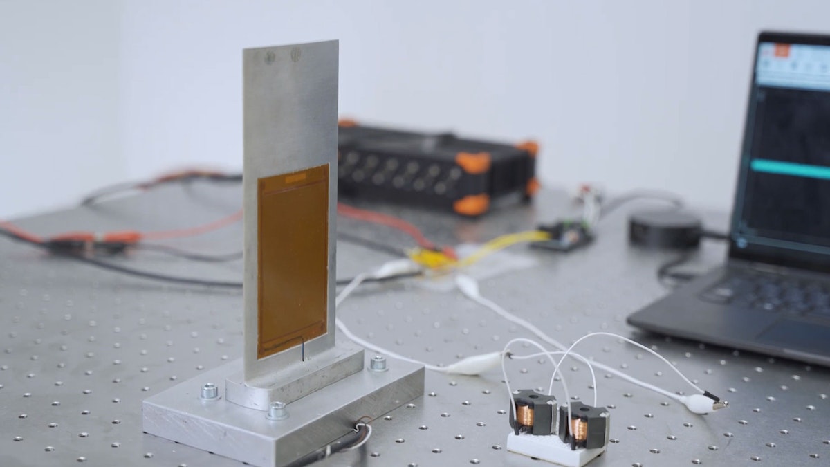
The hydrofoil has two piezoelectric patches to control the bending on one side and a patch on the other to control the torsion. In this experimental setup, we use one of the two "bending" patches as input excitation and the second "bending" patch as sensing output. The input is an excitation voltage, and the output is the voltage across the electrodes of the sensing patch.
During the experiment, we measured the FRF in both the short-circuit case and the open-circuit case, and the dynamic behavior of this plate will be different because of the piezoelectric patches.


The excitation type chosen for this experiment is ‘chirp.’ We based this choice on the fact that a chirp signal can encompass a wide range of frequencies, allowing for studying the frequency response across an extensive frequency range with a single excitation.
A chirp signal is a type of signal in which the frequency increases or decreases over time. It’s commonly used in applications like radar, sonar, communications, and vibration testing because it allows the measurement of a system’s response across a wide range of frequencies. The smooth sweep from low to high (or high to low) frequencies makes chirp signals effective for identifying how different frequencies affect a system or environment.
List of data acquisition hardware and software
For data acquisition and analysis, we used:
DEWE-43: It is a versatile 8-channel USB data acquisition system. The hand-size device has eight universal analog inputs, eight digital/counter/encoder inputs, and two high-speed CAN bus inputs.
DewesoftX: DewesoftX is data acquisition and signal processing software for signal measurement, data recording, processing, and visualization in numerous test and measurement applications across all markets.
Two groups of FRF data are obtained by disconnecting and connecting the two electrodes of the “torsion” patch, corresponding to the open and short circuit cases. We will study two peaks:
The first vibration mode (bending) occurs at the frequency of around 98 Hz;
The second (torsion) appears at around 520 Hz.
We extracted the FRF around 500 to 540 Hz for a more detailed result for the second mode. Figure 2 indicates the results of the short circuit case and open circuit case.


After measuring the FRF data, we need to calculate the piezoelectric capacitance. To avoid the influence of mode shapes, we measured the capacitance in a frequency away from modes 1 and 2. The capacitance at 1000 HZ is 13.62 nF, measured through a capacitance meter.
Then, to find the exact value of mode 2's natural frequency, we implemented the Rational Fraction Polynomial (RFP) method and analyzed data obtained in DewesoftX.
We received the curve fitting and natural frequency results by running the RFP and orthogonal functions. Figures 3 and 4 show the FRF synthesized from the RFP method for both short and open-circuit cases, which correctly approximate the experimental FRFs.


In the next step, we can extract the natural angular frequencies in short and open circuits through the relation:
Hence, we can determine the required optimal inductance L and resistance R using the equations.
Natural frequency (short circuit) = 518.4547 Hz
Natural frequency (short circuit) = 520.4007 Hz
Natural angular frequency (short circuit) = 3.2575e+03 rad/s
Natural angular frequency (short circuit) = 3.2698e+03 rad/s
Coupling factor = 8.67%. Inductance = 6.9 H. Resistance = 2388.5 Ω
The coupling factor reveals the difference between short and open circuit conditions. The plate responds at a slightly higher frequency when in an open circuit than in a short circuit. This variation indicates that the electrical boundary conditions significantly influence the mechanical vibrations of the hydrofoil.
Design and realization of the passive inductor
As seen in Figure 5, a passive inductor's structure consists of four parts: core, coil former, coil, and clamps. In this session, the core type is RM (from TDK Electronics), and the coil is copper wire.


After learning about the structure, we focus on the inductor's inductance, resistance, and filling factor. The inductance value is directly dependent on the number of turns and the magnetic circuit's permeance, derived from the formula with as the permeance and N as the number of turns.
In our case, the inductance is 6.9 H. The data from TDK Electronics give the value of permeance. Each type of RM will have several different permeance values. We can obtain the number of turns from the formula.
Secondly, (series resistance) models copper losses in the wire, and (parallel resistance) models iron losses in the magnetic circuit, see Figure 5. We neglect the parallel resistance in this case and then define the resistance as:
is the resistivity of copper, which equals 17.2 µΩ.mm. 𝑙𝑁 is the wire's length defined by different types of RM cores, and is the wire's cross-section. Then, we introduce the filling factor,
Where is the winding cross-section value, which depends on the coil former. Since the filling factor is usually around 0.5, this value helps define a suitable wire diameter. The resistance can also be calculated by:
also depends on the coil type. If we do the calculation, \(RS\) and \(R_CU\) should have similar results.
In the next step, we calculate the diameter of the corresponding core type used to make the inductor. We can use the Matlab code in Figure 6 to estimate the number of turns, the cross-section area, the series resistance, the resistance , and finally, the diameter of the wire. In this case, the calculation of both and is to check whether these formulae are equivalent.

.")
The objective is to find a solution we can fabricate considering the diameter of existing copper wires:
The first solution uses RM14, un-gapped material PC200. In this case, the theoretical series resistance is 75.28 Ω, and the resistance using a 0.2mm copper wire diameter is 70.84 Ω.
A second solution uses RM12, ungapped material N87 (or N97). In this case, the theoretical series resistance is 37.30 Ω, and the resistance using a 0.2mm diameter copper wire is 38.04 Ω.
A third solution is to use two already available RM10 inductors with inductances of 1.5 H and 6.0 H and resistances of 72 Ω and 325 Ω. This solution provides a relevant high resistance and can be coupled with two 1000 Ω resistances to fit the optimal resistance of the previously defined resonant shunt.
Implementation of single-mode resonant shunts
We implement the solution with the two inductors and study several frequency responses in different cases. The objective is to first obtain the frequency response around the second natural frequency of the hydrofoil without inductors. Then, we add the inductors to the circuit and compare the results. Finally, we will make several resistance and inductance adjustments to fit the optimal parameter obtained previously.
Firstly, we measure the frequency response without the inductors by voltage/voltage FRF in the frequency range of [470, 570] HZ. We use this result as a reference for comparison after connecting the inductors.
Secondly, we implement the inductor circuit, with the total inductance being 1.5 H + 6.0 H = 7.5 and the total resistance being 72 Ω + 325 Ω = 397 Ω.
Then, we obtain the frequency response data (voltage/voltage) both without and with inductors.
See the result in Figure 7 through Matlab plotting.

The result of the original frequency response is satisfactory, as we can observe the peak in the figure. We also see the strong effect of the resonant shunt thanks to the FRF obtained with the inductor.
However, those results are difficult to read because setting the voltage as the output might cause some difficulties in evaluating the adequate tuning of the shunt. Therefore, in the following experiments, we use acceleration as the output to study the details of the structure’s dynamic behavior.
After adding an accelerometer to the experimental setup, we obtain the new frequency response data in Figures 8 and 9.


These two figures suggest that the inductors significantly decreased the structure's vibration amplitude around the second natural frequency. Nonetheless, the inductors' resistance is lower than the target resistance, which is 2388.5 Ω. We use Matlab to plot the data exported from the DewesoftX software and to compare the results.
We added two extra 1000 Ω resistances to fit the optimal resistance. Figure 10 shows the result in the cases 1) without inductor, 2) without resistors added in series with the inductors, and 3) with 2000 Ω added in series with the inductors.

If the circuit resistance is not close to the optimal value, the structure's response becomes two peaks with medium heights. After adding the extra resistance, the circuit's resistance becomes 397Ω + 2000Ω = 2397Ω, which is close to the optimal resistance value of 2388.5Ω.
With optimal resistance, the dynamic response minimizes over a broad frequency range compared to the case with 397Ω.
We added extra resistance to study how the resistance affects the FRF. Moreover, the two peaks in the optimal resistance case are not aligned on the same horizontal line. We might be able to improve this by adjusting the inductance value.
In the next step, we thus compare optimal R, surplus R, and optimal R & L cases. Figure 11 shows that extra resistance recreates the peak in the natural frequency range. We also see that the inductance value can affect the height balance between two peaks around the frequency response.

Conclusion
The resonant shunt can significantly improve the structure's dynamic behavior around a specific mode. We can enhance the damping performance with the proper inductance and resistance, which are close to the optimal values calculated in theoretical ways. The effect of resistance could impact the height of peaks. A lower-than-optimal value results in two higher peaks, and a larger-than-optimal value recreates a single peak.
Finally, the inductance value can affect the balance between the two peaks. These tuning possibilities offer great perspectives for vibration mitigation of mechanical structures in different applications, including air or hydrofoils subjected to flow excitations.