Measuring Wishbone Deformations on an FSAE Car

Superior Engineering is a young and ambitious team. It has over 30 students from different fields. These fields include mechanical engineering, electrical engineering, economics, and natural sciences. Through hard work and support from sponsors, they create chances for technical and personal growth. Our goal? To build and test a formula race car in the Formula Student competition – an international event where all our efforts pay off on the racetrack.

Every year, the Superior Engineering team at the University of Ljubljana puts in a lot of effort. They aim to build the best and fastest race car. They follow the competition rules. This year, our suspension team is working on a project. We are making the steel wishbones lighter and stronger. Our future goal is to replace the steel tubes with carbon fiber ones. 

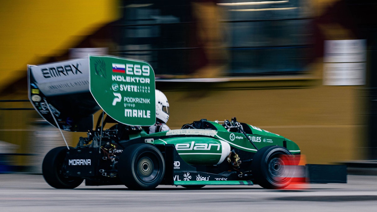
Our 7th racecar, Morana, is powered by two Emrax 188 motors, which can provide 80kW of power together. The car has a separate suspension with front and rear anti-roll bars. This allows for quick suspension adjustments. The vehicle's mass is 209 kg, which can accelerate up to 2g. The team visited four races in 2023 (FS Netherlands, FS East, FS Germany, and FS Alpe-Adria. 

Issue and purpose

To better understand the loads on the wishbones, we decided to measure the deformations or forces in these components. We measured the changes in the tubes using rosettes from TRCPro d.o.o. We connected these to the Dewesoft MINITAURs data acquisition system. 

This is an 8-channel data acquisition system and data logger. It has signal conditioning and supports analog, counter, and CAN inputs.

We conducted deformation measurements in the suspension wishbones and steering rods of the race car with the aim of:

• Validating calculations

• Optimizing the weight of the wishbones

• Measuring torque on the steering wheel

"If you can’t measure it, you can’t improve it." (Peter Drucker)

Theoretical introduction

Every tangible object deforms to some extent when exposed to a force. Specific deformation [ε] is the ratio of the change in length [l] to the initial length [l0] of the object in question.

Resistive strain gauges can measure deformations. These are small and thin gauges made of non-conductive foil, with a conductive wire arranged in a spiral. In an appropriate bridge circuit, strain gauges can measure tension, compression, torque, or temperature changes. 

When the strain gauge sticks to an object's surface, it bends when a load is applied in the right direction. This change makes the wire in the gauge longer or shorter. This, in turn, affects the wire's resistance. Ohm's law states that changes in resistance [R] affect the changes in voltage [U]. This means we can measure deformation by looking at the change in voltage.

With the known size of the object, we can calculate the force on it using Hooke's law. This is true if we take measurements within the elastic deformation range. In the following equation, [E] represents the modulus of elasticity, [F] the external force, and [S0] the initial cross-sectional area of the rod with [] representing the nominal (mechanical) stress.

We can observe that we are still within the linear or elastic deformation range. To be sure, we can calculate the force limit for this range. For a material like 25CrMo4, the yield strength happens at 0.2% strain, or 0.002. By looking at the graph, this corresponds to 410 MPa. Knowing the rod's cross-sectional area (A = 63.617 mm²), we can calculate the limit force using the basic stress equation:

In our case, it is 26083 N, ensuring we are safe within the material's elastic deformation range.

Strain gauges connect in measuring circuits, the most well-known of which is the Wheatstone Bridge. This circuit has four equally connected resistors or strain gauges, with an input Ui (constant) and an output voltage U0.

Based on the number of active resistors or strain gauges, we distinguish between:

• Quarter-bridge configuration, with only one active gauge: This configuration is rarely used as it does not allow us to isolate individual signals from the measurement, and the signal is also affected by temperature changes.

• Half-bridge configuration, with two active resistors: This configuration compensates for temperature changes.

• Full-bridge configuration, where all resistors are active: This configuration compensates for the influence of bending and temperature changes, resulting in a voltage ratio Ui/U0​​ that is linear and dependent solely on the deformation caused by axial force.

Wishbones

The race car utilizes double wishbone suspension. Wishbones are welded tubes of 25CrMo4 (1.7218) material. We measured four pairs of control arms with a tube diameter of 15/1.5 mm and two steering rods with a 12/1.5 mm diameter. Before we attached the strain gauges, we needed to find out how stress was spread in the arms. This helped us choose the best spots for the gauges. For this, we performed a finite element analysis (FEA), considering the boundary conditions of cornering.

The upper control arms, which must transfer forces from the road to the dampers and springs, present a particular challenge. These forces introduce bending into the upper wishbone. 

Through simulation, we identified the locations where we could measure deformation with the least influence of bending deformation. We did a strength analysis using the finite element method. We assumed a vertical load of 1000 N on the tire. We examined how stress and deformation are distributed in the arm. As expected, the stresses were lowest around the neutral axis.

Selection and preparation of measuring equipment

In our case, we chose the full-bridge setup. We only cared about the axial force. We chose HBM strain gauges 1-XY11-3/350 E for the 15 mm diameter steel tubes. We considered these criteria when selecting the strain gauge:

• Suitable size in relation to the size of the measured object

• Appropriate shape for the specific measurement type

• Compatible type of strain gauge with the material of the measured object

• Suitable resistance of the strain gauge

• Appropriate temperature range for the strain gauge

The chosen strain gauges are in pairs on a single rosette. Because steel has the same coefficient of thermal expansion, they are suitable for measurements of that material.

We wanted to measure in a place with stress like uniaxial stress. So, we placed the strain gauge 5 cm from the end of the tube. Before bonding, we made a thin marking parallel to the tube axis on both sides at this location. We used a 3D-printed guide. It was a rectangular block with a 7 mm deep circular groove. This helped us transfer the line to the bottom of the tube. We made sure the rosettes were as parallel as possible.  

Before gluing the strain gauges, we lightly sanded the tube. We also cleaned the surface with acetone to ensure a strong bond. We placed the rosette on a clean glass surface and applied adhesive tape to its back. The tape was then affixed to the tube, aligning the strain gauge with the marked centerline. 

We used a drop of cyanoacrylate adhesive, commonly known as super glue, onto the tube. The advantage of this adhesive is its quick curing at room temperature. We gently pressed the strain gauge onto the surface, wrapped it with Teflon tape, and waited 10 minutes for the adhesive to cure.

We soldered the signal cable from the strain gauges to a TED connector. This connector works with the Dewesoft MINITAUR DAQ system. This system includes an integrated A/D converter, a signal processing module, and a computer running data acquisition software. It has eight analog and several digital inputs, allowing sampling up to 20,000 Hz at 24-bit resolution. 

We selected a sampling frequency of 5 kHz, which provided precise data acquisition while keeping the data volume manageable. We chose this frequency based on the Nyquist criterion. We assumed the race car goes 100 km/h over a 50 mm bump. This creates a signal with a frequency of about 550 Hz. To capture the signal in a short time, we needed a sampling frequency. This frequency had to be 5 to 10 times higher than the interference frequency.

Measuring chain

The measuring chain started with 18 strain gauge rosettes for uniaxial measurements from HBM (type 1-XY11-3/350 E). After gluing the rosettes to the wishbones, we connected them. We used quarter-bridge wiring for the wishbones and half-bridge wiring for the tie rods. 

To provide sufficient signal to the DAQ, we had to make an additional amplification for the half-bridge wiring. We could use a Dewesoft STG amplifier or manually solder additional resistors into the half-bridge wiring. We decided to solder 2 x 350-ohm resistors into the half-bridge wiring manually. 

We then soldered wires to the TED connectors, which were plugged into the Dewesoft MINITAUR DAQ station. After that, we set up all the sensors in the DewesoftX software and executed sensor calibrations. We processed further data for Rainflow analysis in Python. However, there is also an option to do Rainflow analysis directly in the DewesoftX software.

Sensor calibration

After we installed and connected the strain gauges, we got an output voltage. However, this voltage did not directly tell us about the tensile force. We needed to adjust the strain gauges. This would help us find a number to multiply the output voltage. This number would show the real axial force in the tube in SI units. 

We calibrated the sensors at the Faculty of Mechanical Engineering at UNI Ljubljana. We used a servo-hydraulic testing machine in the Laboratory for Machine Elements (LASEM). The calibration was accurate to ±5 N. We gradually increased the force by 400 N until it reached about 3 kN. Then, we released the force in the same steps. This process also lets us check for hysteresis. Hysteresis is when a material responds to forces with a delay. It may not return to its original value after unloading.

The calibration result was a step graph that looked like a pyramid. We used Python code to match it to the actual force applied during calibration. We then saved these results into the DAQ station to obtain the desired tensile force in the wishbones as the output.

Figure 14 shows the settings used for a strain gauge on a specific suspension arm. We entered the offset by inputting two data points from the Python code into the channel setup. The system automatically calculated the offset and calibrated the strain gauge for us.

Measurement and analysis

After calibration, we protected the sensors from the weather with heat shrink encapsulation. Then, we reinstalled the wishbones on the race car. We connected the sensors to the DAQ system and battery, which we had mounted under the driver’s legs. The first test took place at the Student Campus. We set up a track like those used in Formula Student competitions. We tested the load conditions at the highest possible speeds in corners, during full acceleration, and under hard braking.

Forces in the wishbones

The image below shows the measured force values in the race car's suspension, captured over approximately 200 seconds. We expected to find a lot of high-frequency noise in the measurement. So, we used a low-pass filter. The cutoff frequency was set to 40 Hz. This filtering provided a clearer measurement. It also captured the key cycles needed for damage assessment in load spectra studies.

We also observed that the data obtained is very “dense.” We tested on a track with tight corners and short straights, so we couldn’t achieve speeds higher than 70 km/h. Therefore, the sampling frequency could be lower. After cleaning noise from the data and doing more work, it became clear that a sampling frequency of 1000 Hz would be enough. For easier data processing, we used 1000 Hz instead. 

As forces don’t tell much about a component's load capacity, it is better to examine stresses. DewesoftX provides different math tools for offline signal processing. This allows us to calculate axial stresses in the tubes on wishbones. We do this by using a simple formula for each measured force signal.

We decided to do further data processing with the rain flow calculation in Python. However, it is worth mentioning that the DewesoftX software also has the option to do the rain flow analysis.

Using a simple algorithm, we could identify local peaks and valleys—or local turning points from the filtered signal. These served as a basis for further analysis of the load spectra.

Rainflow analysis

In high-cycle fatigue, several methods exist for analyzing load history. One method is Rainflow analysis. It helps us find load cycles from the stress-time signal. We can then calculate how much they contribute to the total damage of a component. This analysis consists of six main steps:

Step 1

We begin by filtering the data to remove noise that may be present in the measurements. Here, we aim to remove only low-frequency noise, as a high-pass filter would alter the signal or load cycles. The signal is typically represented as voltage.

Step 2

Next, we identify local peaks and valleys (peak and valley analysis). These variations provide the signal’s turning points, which are essential for recognizing load cycles.

Step 3

Larger load cycles, or force changes with higher amplitudes, cause the most fatigue damage. Therefore, it is not practical to include smaller cycles that add little damage in the analysis. To achieve this, we divide the stress range in the signal into classes (“binning”).

You must select the class size to filter out small, insignificant cycles without setting it too high. Such a setting would significantly alter the stress amplitudes of individual cycles and, thus, their contribution to the damage. Our load spectrum ranges from +50 MPa to -310 MPa, so we choose a class size of 5 MPa. Figures 21 and 22 show the result of this binning process:

Step 4

Following this is the core part of the analysis—cycle extraction. The algorithm examines four consecutive turning points of the signal. The Rainflow method has these cycle extraction rules:

1. Select four consecutive points in the signal, S1, S2, S3, S4.

2. Calculate the stress difference |S2 - S3|.

3. Calculate the stress difference |S1 - S4|.

4. If |S2 - S3| ≤ |S1 - S4| and points S2 and S3 are within S1 and S4, the cycle is counted.

5. If |S2 - S3| ≥ |S1 - S4| and points S2 and S3 are not within S1 and S4, the cycle is not counted.

For a more detailed explanation of the Rainflow method, please refer to Rainflow Counting.

Step 5

After extracting cycles from the signal, we obtain a load pattern with cycles removed, referred to as the residue. We then duplicate the residue (residue + residue), creating a new pattern for cycle removal. This step captures the most significant load cycles, contributing the most to overall damage. Once we remove these cycles, we can create a Rainflow matrix.

Step 6

This matrix's cycles along the diagonal represent smaller cycles that contribute minimally to total damage. However, the points in the upper left and lower right corners show much larger cycles. These cycles cause a much higher amount of damage. The distribution forms a parallelogram: the narrower this parallelogram, the more significant the proportion of high-load cycles.

Now that we understand the load spectrum of the wishbones, we can estimate how long they will last. We can also check for damage after a certain number of kilometers. The lifespan of a Formula Student race car is about 4 to 6 months. It can cover up to 1500 km. Most FSAE cars usually cover 500 km or less.

The analyzed load spectrum lasts 760 seconds. We covered 10.55 km at an average 50 km/h driving speed during the measurement. To show the full lifecycle load for a vehicle that lasts 1500 km, we must repeat the chosen spectrum 142 times. 

If we have the S-N curve for the material 25CrMo4, we can use Haigh's rule to calculate damage. The S-N curve is used for alternating load cycles with an average stress of 0 MPa. We need to find an equivalent stress for each cycle. This stress will help us in the damage calculation. 

Haigh's rule states that if the equivalent stress of a cycle exceeds the material’s fatigue strength at R = -1 (alternating load), we calculate the number of equivalent load cycles using the following equation:

If the equivalent load is lower than the fatigue strength, we use a specific equation. Set N(D=0) to 2,000,000. Then, use the calculated value for kkk. We calculate the number of load cycles to critical damage for each load cycle using these two equations. With Rainflow analysis, we also know the repetition count of these cycles throughout the suspension's lifespan.

We can use this information to find the damage from each cycle. We can also calculate the total damage over the lifespan. For cumulative damage, we use Palmgren-Miner’s rule of linear damage accumulation. We calculate the damage of each cycle with the following equation:

Where ni  ​ is the number of repetitions of a load cycle, and Ni  is the number of cycles to critical damage for a selected cycle. The following equation calculates the total contribution to damage:

Considering one repetition of the analyzed load spectrum (10.55km), its contribution to the damage is 1.43∙10-5 =0.00143%. After 1500 km or 142 repetitions, the contribution to the damage is   2.0306∙10-3 = 0.203%.

Moment on the steering shaft

We obtained the force by measuring the deformation in the steering rod, allowing us to calculate the steering shaft moment using the equation below. If we had data on the steering angle, we could consider the universal joint’s effect. However, we could not record data from both sensors at the same time. The moment, based on the known force, is calculated as follows:

The angle between the rack and the steering rod changes as the wheel turns, but since the maximum angle is 8°, we can use the small-angle approximation: cos⁡(θ)≈1\cos(\theta) \approx 1cos(θ)≈1.

As with the suspension force measurements, we used a low-pass filter with a cutoff frequency of 50 Hz here. The filtered data, free of noise, is shown below. Significant disturbances remain in the signal, which we cannot fully explain. We made the measurements at a frequency of 1000 Hz.

We also measured the moment on the left tie rod alongside the right one. We then used the equation to calculate the moment on the steering shaft, which appears in the program as follows:

The graph in Figure 29 shows the result of the moment calculation using the above function. For an FSAE race car, the recommended steering wheel torque, in turn, is between 5 and 10 Nm (according to Claude Rouelle). In our case, however, the moment sometimes rises to 25 Nm, nearly 2.5 times the recommended value. This number supports the drivers' comments about the hard work of turning the wheel. This difficulty leads to quick driver fatigue. It also makes it hard to keep steady lap times during longer races, like the Endurance discipline.

We will change the front suspension setup next season. This will help reduce the moment. We will focus on the caster angle. The caster angle affects the distance known as the mechanical trail. This change affects the lever arm of the lateral force from the tire. It acts around the wheel’s rotation axis, creating a moment around that axis. 

Reducing this moment can decrease the force in the steering rod and, consequently, the steering wheel torque. If the dimension of the steering rack pinion is modified, we will also have to consider this effect.

Conclusion

The measurements have given the team a lot of new knowledge. We can use this to improve components and better understand the suspension loads. We optimized the wishbone tubes from a diameter of 15/1.5mm to 14/1 mm using the same material (25CrMo4). Measurements have also served as a basis for researching adhesive joints for CFRP wishbones. 

Measuring deformation in the pushrod can give important data on tire forces. This helps us check our tire model and use grip effectively. To achieve this, we would need additional sensors and an IMU sensor. However, with the combination of an IMU, a steering angle sensor, and knowledge of ride height (measured via suspension angle or ride height sensors), we could gain excellent insights into grip utilization, which is critical for performance.

We want to thank Dewesoft for their support. Access to cutting-edge measuring technology benefits us as a team and as students regarding competencies. 

We’d also like to thank HBM Corporation and TRCPro d.o.o. for sponsoring us with 20 rosettes (strain gauges). Without their support, the measurements would have been impossible. 

References and literature

1. Brecelj, Matevž. Razvoj merilnega sistema za merjenje sil in zasukov v podvozju vozila Formula Student. Univerza v Ljubljani, Fakulteta za strojništvo, 2020. 

2. Cingerle, Alen. Razvoj krmilnega mehanizma za dirkalno vozilo Formula Student. Univerza v Ljubljani, Fakulteta za strojništvo, 2020.

3. Nagode, M. (2024). Zapiski predavanj obratovalna trdnost. Univerza v Ljubljani, Fakulteta za strojništvo

4. Mechanicalc. (n.d.). Beam analysis. Pridobljeno oktober 22, 2024

5. Siemens. (n.d.). Rainflow counting. Retrieved October 24, 2024

E. A. A. Mohamed, M. A. Yusuff, and D. A. Wahab, "Application of Rainflow Cycle Counting in the Reliability Prediction of Automotive Front Corner Module System," in Proceedings of the International Conference on Industrial Engineering and Engineering Management, Beijing, China, 21-23 Oct. 2009, from: Application of rainflow cycle counting in the reliability prediction of automotive front corner module system | IEEE Conference Publication | IEEE Xplore. DOI: 10.1109/ICIEEM.2009.5344498.