


Measuring Frequency Response Function (FRF) To Characterize Structure Dynamics on Racecar Chassis
Christian Cicala (Mechanical Engineering Student)
University of Trieste
October 5, 2023
The frequency response function (FRF) is the bread and butter of every person involved in system dynamics. The FRF function is simply the ratio of the system’s output response due to an applied excitation. Engineers use FRFs to measure and characterize a structure’s dynamic behavior.
The measurement of Frequency Response Function (FRF) is the basis for the Experimental Modal Analysis (EMA). Frequency response measurements lead to identifying a higher quality of modal parameters.
A good frequency response function should at least:
have decent frequency resolution and frequency span,
contain all the structure’s resonances and through this modal shapes in the band of your interest, and
have good coherence (>0.9 at resonance frequencies).
In modal testing, engineers usually make FRF measurements under controlled conditions. The test structure is then artificially excited by either an impact hammer or vibration shaker(s) driven by broadband signals. Selecting the structure’s excitation and response points is crucial for the EMA. The pre-test analysis can provide convincing advice on designing an appropriate modal test if you don't know where to start.
Below, I show how I measured FRFs in different modalities and used the pre-test. Let's start right from the latter!
The object of my dynamics analysis was the Formula SAE racecar chassis owned by the UniTS Racing Team - see Figure 1.


Pre-test analysis
Using the pre-testing analysis can lead to the measurement of higher-quality FRFs. The pre-test tools can post-process the Finite Element Analysis (FEA) results and derive information for planning and optimizing experimental tests. Below are typical pre-test activities.
Optimal sensor location selection
The basis of location selection is the ability of a sensor set to capture modal shapes. If not correctly positioned, one or more modal information may be missed (spatial aliasing). Correct positioning makes it possible to avoid nodal lines - points that do not move - in the structure.
Optimal selection of the position and direction of the excitation points
In the case of shaker tests, the location of the excitation should be at a rigid point in the structure. This way, the kinetic energy feds into the system.
Optimal selection of the suspension points of the structure
The structure should be supported so that the set-up has minimal impact on its modal shapes. Such setup is done, e.g., by suspending it at the points with the lowest modal displacement or kinetic energy.
However, be careful! Although pre-testing tools are a great help, the experience of the engineer performing the test remains a crucial resource in deciding the best strategy.
I identified 26 points of excitation/response on the structure. I discovered that the supports could be attached to nearly any part of the structure except the Main Hoop. I suspended the frame on a rigid support system using elastic ropes - see Figure 2.


However, there is no free meal. As well as the pre-test, FEA is required. After the boring initial part of the testing spent on the PC - let’s start to measure some FRFs!
Frequency response function with impact hammer test
One of the simplest methods of measuring FRF is the impact hammer test. An impact hammer excites the structure by short pulses while one or more accelerometers measure the response.
The hammer has an integrated force sensor and interchangeable tips with different stiffnesses. The excitation frequency range is determined primarily by the stiffness of the hammer tip. The harder the hammer tip, the wider the excited frequency range. The selected hammer tip must excite all modes in the considered band of interest - see Figure 3.


The output and the measured Frequency Response Functions (FRFs) for various inputs correspond to the measuring elements taken from a single FRF matrix row. Typical of a roving hammer impact test - see Figure 4.


Measurement setup
I used an impact hammer with a semi-hard tip and five single-axis accelerometers to carry out the test. The accelerometers were attached to the structure by magnets to ensure stable positioning - see Figures 5, 6, and 7.


I used Dewesoft’s KRYPTON-8xACC data acquisition system (DAQ). It is an 8-channel IEPE/Voltage input module (Figures 8 and 9). KRYPTON DAQs are bundled with DewesoftX software to process and analyze the data.


I set the following parameters in DewesoftX:
Sampling frequency (fs): 1000 Hz, corresponding to a bandwidth of 391 Hz.
Sensitivity of the hammer load cell: 10 mV/N.
Accelerometer sensitivity: 10 mV/(m/s2).
Resolution: 0.244 Hz, for an acquisition time of 4.1 s.
Roving hammer - specifications.
Linear average - over three hammer hits per excitation point.
Estimation H1 of the FRF.
Trigger level 10 N, Pre-trigger 1%.
Force and Exponential Window - window length 6%, window decay 5%: I used the force window to remove noise from the pulse signal and the exponential window to reduce leakage in the response spectrum.
In the Geometry editor, I defined a cartesian reference system. Based on this, I constructed the frame geometry using the 26 points – see Figure 10. I took care to orient these in a way that the hammering would not be parallel to the reference system.


Figure 11 shows two FRFs measured by hammer test. The peaks with a relatively high coherence value represent the resonances of the system and are visible for all measured FRFs. In the figure, it is also possible to observe the measurement on a nodal point in pink FRF.


Resonance or natural frequencies are not present at the beginning and end of the band, which results in not fully capturing the structure’s modal shapes. At that point, the measurement direction represents a node for low-frequency and high-frequency modes.
The amplitude of the peaks is higher than in the green FRF as the modes present in the pink FRF will be predominantly along the X direction. When performing a modal analysis, all structure modes in the band of interest must synthesize all other FRFs the best! Pay attention to the completeness of the measured FRFs!
The theory says the FRF matrix is symmetrical. In experimental measurements, I must consider both - the sensor and the excitation direction. These can lead to an imperfect match of the matrix’s symmetric elements, as shown in Figure 12.
I explain this by the very high hammer crest factor. For a short period, so much energy concentrates on a small area of the structure. This energy excites the structure’s nonlinearities, which leads to a mismatch of the symmetric elements of the FRF matrix.
If the structure is strongly nonlinear, a shaker test may be the best option!


Frequency response function with shaker test
You cannot use an impact hammer test to measure FRFs on all structures. The alternative method is using the vibration shaker to perform the test.
Engineers use modal shakers to excite large or more complex objects and to obtain high-quality modal data. Shakers can, in comparison with modal hammers, excite structures over a broader frequency range. They can also apply a range of signal types depending on the structure type - see Figure 13.


The shaker is usually attached to the structure using a stinger. The stinger is a long, thin rod - see Figure 14. It can only transmit a force along the axis of the stinger to the system.


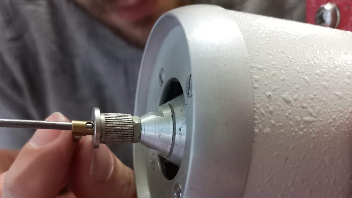
A load cell between the frame and the stinger can measure the excitation force - see Figure 15.
The stinger is subject to buckling, so the rod stiffness must be sufficient to keep it from bending during the excitation phase.
Measurement setup
I used a stand - see Figure 16 - to bring the modal shaker on level with the desired point on the chassis. Node 4 was chosen as the excitation point since it is a rigid point of the structure that is easily accessible.
I decided to proceed as follows. To make the results more comparable, I oriented each sensor on each structure point to coincide with the excitation direction at the same points used in the hammer test.
I used five single-axis accelerometers attached to the frame by magnets. Dewesoft's 16-channel SIRIUS DAQ system - see Figure 17, enabled the connection of the shaker power amplifier - see Figure 17. The data were analyzed using the DewesoftX data acquisition software.


I performed all shaker tests by setting the following parameters on the software:
Sampling frequency (fs) - 1000 Hz, which corresponds to a bandwidth of 391 Hz.
Sensitivity of the hammer load cell - 10 mV/N.
Accelerometer sensitivity - 10 mV/(m/s2).
Resolution - 0.25 Hz for an acquisition time of 4 s.
Estimation H1 - the FRF.
Excitation source to ’Dewesoft analog output’ and Analog output soft start/stop time to 0.5 s.
Analog out amplitude 1.00 V.
Geometry remains the same as in the hammer test.
I did three tests by selecting different types of excitations:
Continuous random
Burst random
Sine sweep
Continuous Random
The analog out channels emit continuous random noise having a bandwidth equal to half the sampling rate. In Continuous mode, the software continuously calculates spectra when acquiring data during the measurement. During the test, I stopped the calculation when reaching 150 Spectra. I used the ‘Blackman’ time-weighting window with a signal overlap of 50%.
Burst Random
The structure is excited by random signals. The burst length is user-defined. The burst duration can be defined through the ‘excitation duration’ parameter. I specified the excitation duration as a percentage of each spectrum’s FFT time block length. In this case, 50%.
Random Bursts will have a bandwidth equal to half the sampling rate of the DAQ device. This type of excitation doesn't require using a weighting window because the signal inherently lacks leakage and behaves like a transient signal. To guarantee this, limit the excitation duration to fall within the time block of the FFT, which also includes the analog out soft start/stop times.
Sine Sweep
The structure is excited by a sinusoidal signal crossing all frequencies from a ‘Start freq’ to a ‘Stop freq’ within a sweep time. The sinusoidal sweep test generally provides great consistency between input and output. The total excitation force supplied to the structure can be kept relatively low since only one frequency is excited at a time.
In addition, the sweep time must be long enough because the FFT needs some time to compute depending on the number of spectral lines and the resolution. In this case, I set Start freq. at 5 Hz, Stop freq. at 450Hz, a Sweep time of 300 s, and the Blackman-type time-weighting FFT window with a Signal overlap of 50%.
Figure 18 shows the FRFs measured with the three different types of excitations. A good overlap of the FRFs is evident. The Burst Random peaks have a slightly larger amplitude, probably because I didn’t use a weighting window.
The coherence of the FRF obtained by the Sine Sweep is the best of the three, while Burst Random is the worst. In low-damping structures, in the case of excitation with Burst Random, reducing the excitation duration can provide better coherence.

, Burst Random (red), and Sine Sweep (blue).")
In Figure 19 I compare the FRFs obtained with the hammer and the shaker. Note that in the FRF obtained through the modal hammer, all first modes of the structure are present in the first half of the band.
In the second half of the band, the best completeness of the structure’s modes is obtained with the shaker. The trend of FRFs obtained with the shaker is more constant. Also, note that the amplitude of the FRF obtained by the hammer test is lower than the others, probably due to the nonlinearity of the structure, which particularly stands out when excited through the hammer on that point.

, shaker Continuous Random (yellow), shaker Burst Random (red), and shaker Sine Sweep (blue).")
To conclude, I obtained two good-quality FRFs by shaker and hammer testing. In this case - see Figure 20, the two FRFs match and show a constant trend with good peak separation. The hammer coherence, in this case, results better than the shaker.


Conclusion
In conclusion, I used a pre-test, and various FRFs were measured using different excitation methods. I compared the FRFs, highlighting the peculiar differences.
It’s not a simple matter to obtain quality FRFs, but increased measurement consciousness, which is also obtainable through pre-testing, will lead to better results!
After measuring FRFs, I can use the DewesoftX Modal Analysis module to finish the EMA.
Bibliography
Dewesoft online PRO training
Avitabile, Peter: Experimental modal analysis - A simple non-mathematical presentation. University of Massachusetts Lowell, the USA, 2001.
Brandt, Anders: Noise and Vibration Analysis: Signal Analysis and Experimental Procedures. Wiley, 2011.
Sani, Shahrir & Rahman, Prof. Dr. Md. Mustafizur & Noor, M.M. & Kadirgama, Kumaran & Nor Izham, Mohd Hafizi: Identification of Dynamics Modal Parameter for Car Chassis. University Malaysia Pahang, 2011.
Schwarz, Brian, and Mark H. Richardson: Experimental Modal Analysis. Vibrant Technology, Inc. Jamestown, California, 1999.
Wang, E., Zhou, H., and Zhu, L.: The application of pre-test analysis in modal test. 2nd International Asia Conference on Informatics in Control, Automation and Robotics (CAR 2010), Wuhan, China, 2010.