


Testing Powertrain on an Electric Formula SAE Car
Antonio Maria Pisciotta, Agostino Formisano, and Francesco Giuseppe Quilici
E-Team Squadra Corse
January 30, 2025
The Italian Formula SAE team, E-Team Squadra Corse, has participated in the SAE Formula Student competition since 2008. The 2022/23 season saw a drastic change for the team: Two axial flux motors replaced the well-known internal combustion engines. Switching the powertrain from ICE to electrical proved to be a tough challenge. The team collaborated with Dewesoft to acquire, process, and analyze test data to clarify the consequences of this change on the car's behavior.
In the 2023 season, the E-Team from the University of Pisa made a change. They switched from the combustion category to the electric category in the SAE Formula Student competition. To support this change and improve the engine, our powertrain and electronic teams worked together. They installed and monitored all the vehicle's electronic and electrical devices. To switch to an electric car, we had to change the rear chassis of the single-seater. This change allowed us to attach the new powertrain and battery pack.
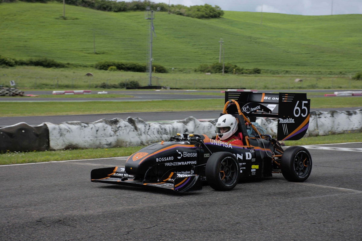
The EV-A vehicle
The first electric car of the E-Team and Ateneo Pisano is E-VA. It has a hybrid chassis. The rear is made of a steel truss, and the front is a carbon fiber monocoque. The car's propulsion system has two rear motors from the aircraft. Each motor is paired with an inverter. This setup connects the motors to the battery.
The E-Team Squadra Corse tested their electric prototype, named ET15: E-VA. They did this at the Circuito di Siena. This international karting track is located in Castelnuovo Berardenga, in the province of Siena, Tuscany, Italy.
| Specifications | Abbreviations | Numerical values |
|---|---|---|
| Mass (car+driver) | m | 336 kg |
| CoG height | h | 300 mm |
| Wheelbase | l | 1530 mm |
| Front track | t1 | 1235 mm |
| Rear track | t2 | 1146 mm |
| Weight distribution (% front) | wb | 45 |
| Front no roll center height | q1 | 12 mm |
| Rear no roll center height | q2 | 34 mm |
| Power | Ptot | 74 KW |
Sensor setup
The installation on the car includes both sensors owned by the team and some provided by Dewesoft.
The team’s sensors
The team owned and had already mounted Internal sensors on the prototype. Typically, we equip the vehicle with:
Throttle position sensor (TPS), which measures the position of the throttle pedal and is potentiometer-based;
The steering position sensor (SPS) connects to the rack. It helps calculate the steering angle of each front wheel based on how the steering moves;
four Hall sensors, one for each hub, measuring the angular speed (ωij) of each wheel ;four potentiometers, one for each shock absorber, measuring their stroke.


The Dewesoft sensors
The external sensors are state-of-the-art, manufactured and supplied by Dewesoft, and are:
SIRIUS Modular - a versatile and robust data acquisition system providing high-end signal conditioning amplifiers for signals and sensors;
DC-CT Current Transducers - providing the advantages of a zero-flux current transducer but with lower power consumption and a more compact design;
Current transducers - current clamp high-accuracy sensors for AC/DC measurement;
Voltage sensors;
DS-GYRO3 is a high-performance inertial measurement unit (IMU). It is firmly attached to the vehicle frame. It is placed as close to the center of gravity (CoG). This unit measures acceleration in longitudinal, lateral, and vertical directions. It also measures the installation point's roll, pitch, and yaw rates.


Vehicle dynamics
Thanks to the IMU from Dewesoft, we could get important vehicle dynamics data that is usually hard to obtain. First, we check that the data are consistent and have the right signs. Figure 2 shows the vehicle model taken as a reference.
The first important step was to compare the signals from the Dewesoft hardware with those from the internal hardware.
As can be seen from Figure 3, the beginning of the acquisition was not synchronized, causing a clear time shift of 127.6 seconds. However, this synchronization was possible thanks to the double acquisition of the throttle signal. The signals are superimposed, as shown in Figure 4.


The next step was to verify that signals had the same signs. To do this, we considered Figure 3. We compared two signals, one with a particular sign, in this case, the steering angle, as a reference and another. We needed to check that the steering, lateral acceleration, and yaw rate were aligned to have the correct signs. Figure 5 shows that ay and the steering angle have opposite signs, so it is necessary to flip ay.
The last comparison involved steering wheel angle and yaw rate, which, as shown in Figure 6, have the same sign and are correct.


Signal processing
To begin with, we extrapolated a single lap from the required data. We achieved this extrapolation by using numerical integration of the yaw rate. From this, we found the positions in the yaw angle vector for values 2π and 4π (see Figure 7).


We obtained the trajectory by exploiting the COG velocities and yaw rate sampled directly from the IMU and integrating eq. Eq. (1) to get absolute x and y data, as shown in Figure 8.


Mechanical analysis
Developing a high-performance prototype vehicle requires an advanced study in vehicle dynamics that improves lap time performance. Over the years, technology has helped create better vehicle models. These models let us predict how vehicles will behave more accurately. However, these models require a correlation between simulated and actual measured data. Thanks to Dewesoft, we can acquire signals with a more precise resolution.
Vehicle model
The vehicle dynamics division has developed various vehicle models. In this case, we validated the multibody model developed using the commercial software Adams Car. The model in Figure 9 has 13 degrees of freedom. These are related to the movements of the sprung mass, unsprung masses, wheel rolling, and the differential.


Three primary levels compose a vehicle model:
Templates, parametric models built in DewesoftX Template Builder expert mode that define topology and significant roles of models;
Subsystems that are in DewesoftX Standard Interface based on templates and are modifiable via parametric data (i.e., suspension coordinates);
Assemblies include all the subsystems needed to define the vehicle. They may also have a test rig to simulate any standard or custom maneuver.
The team created templates for each main vehicle area. This included the front and rear suspensions, steering, chassis, wheels, brakes, and drivetrain. By changing the relative parameters, like the suspension geometry, we can see differences between the 2023 and 2022 models.
The first step in checking our subsystems is to see if we applied all the constraints correctly. Then, as shown in Figure 9, we analyzed some kinematic characteristics of a suspension assembly.
Static validations
The Adams Car model includes elastic connections (bushings) between the suspension triangles and the chassis. In the software, the Adams Car bushing uses a 6x6 matrix, where six generalized displacements and velocities serve as inputs, producing a generalized force vector as output.
For this vehicle, we set the rotational values to 0 based on the connection type used. Additionally, we assumed isotropic behavior for the bushings, meaning the generalized forces act equally in all three directions.
We used strain gauges thanks to a test campaign with Dewesoft in previous years. These gauges measured the deformations of a tie rod during a tensile stress test. The strain gauge was necessary. It helped to distinguish between the arm's deformation and the deformation of the connecting links at the rod ends.
The measurement setup is a half-bridge with two other resistors simulated through amplification. This setup allows us to have a virtual full bridge. We did the static test setup using a car push rod and SKF M6 ball joints; Figure 10 shows the setup. The tie rod connects to the machine through two jaws and with calibrated screws between the jaw and the ball joint. The acquisition was possible through a homemade BNC connector soldered to the cables of the amplification system. We made the calibration with a push rod mounted on a machine from which we took the reference. Once calibrated, 2KN was applied.


The results we got are linked to the whole pushrod assembly. We used interpolation, as shown in Figure 11. This process enabled us to create the .bus file to be inserted into the software, as shown in Figure 12.


Strain gauge test
Once the law of elastic connections was derived, we analyzed dynamic tests made in collaboration with Dewesoft. In 2022, we conducted a test campaign in which we instrumented the suspension arms with strain gauges. This instrumentation allowed us to derive all the through-loads from the suspension arms. Compared to 2024, the car featured a combustion engine in 2022. Table 1 shows the vehicle data.
These tests verified that the forces measured by the software were consistent with what we measured. The study concerns an acceleration and braking maneuver. Figure 13 compares the model and longitudinal acceleration and forward velocity measurements.

Figure 13 shows that the kinematic part matches the measured behavior. Some oscillations are due to vibrations and noise during data collection. Next, Figure 14 shows the team’s internal nomenclature to define the constraints used by the suspension. With the definition of the nomenclature, it is possible to interpret the results shown in the following figures. The results here are associated with the left front suspension.


The results show that the forces' trends tend to be accurate but do not always coincide perfectly. This imperfection is due to two factors:
The modeled road is a smooth plane in the software,
The modeled bushing's viscous characteristic has a linear pattern.
A more in-depth study of its behavior, which we will do in the future, can provide a clearer picture.
Track test campaign in Siena
After the test campaign in 2022, we will proceed in 2024 with the analysis of the mechanical part of the test done in Siena. In this case, the car has an electric motor, and Table 1 shows its characteristics.
Thanks to DS-GYRO3 IMUs, we could measure amounts that are usually hard to get. The test day included three main runs:
4-5 laps for rider training
Mini runs like AutoX to evaluate maximum performance
An endurance run of 22 laps


‘For validation, we took lap 7 of the AutoX run. We wanted to look at the key measurements for a vehicle. These include accelerations and speeds in the vehicle's plane, as well as the speeds of all four wheels. Due to problems during the acquisition phase, evaluating the travel of the four shock absorbers was impossible. Figure 17 shows the results.


The signals are all consistent between simulated and measured. There are minor discrepancies in the signal of the left rear wheel because, in that phase, the lateral load lifts the wheel. To complete the validations, we compared the rack's movement signals.


In Figure 20, it is possible to verify that the trend is the same, with slightly lower peaks. We can attribute these to a tire formulation underestimating slip angles with the same vertical load and lateral force. This underestimation may be due to a less-than-perfect asphalt condition on the day of the tests.
Despite minor discrepancies, this test campaign made it possible to consider the vehicle model validated. From now on, we can use the model to design our future vehicles.
MAP approach
The MAP approach (Map of Achievable Performance) can present a study of our vehicle's handling characteristics.
Ideally, all-time derivatives, forward, lateral, and yaw localities, are zero during a steady-state maneuver. In practical terms, the vehicle drives along a constant-radius circular path at a constant forward speed. When you repeat the process for multiple values of forward speed, you can determine achievable regions and handling characteristics.
The complete model is created by combining all the defined subsystems. It is launched using several maneuvers from the open-loop steering events. This includes ramp steering, as shown in Figure 21. The ramp is slow and takes place over a long time.


A. MAPs β - ρ
Two variables, vehicle slip angle and center of velocity lateral distance, are respectively defined β and ρ, which is the CoG curvature in the steady state condition described in the equation:


The MAP β - ρ shows how the vehicle handles. In Figure 22, the yaw rate r usually matches the steering angle's sign. However, this is not true for the lateral velocity v. It is worth noting that vehicle characteristics here, given a constant speed, change sign with a variation of curvature. Furthermore, at low speeds, β and ρ have the same sign; this behavior is often called nose-out. The opposite goes as the speed increases, giving a nose-in behavior.
Other MAPs help understand the under-oversteer concept better.
B. MAPs ρ - δv
Vehicle dynamics focuses on studying the vehicle's behavior in response to the driver’s input. The plane (ρ, δv ) can represent this relation well - see Figure 23.
It is clear that some constant forward speed curves reach a limit as the steering input increases. This instability may show that the vehicle tends to understeer.


C. Input Achievable Regions
The input MAPs u, δv, and ãy can help understand the vehicle limits regarding achievable lateral acceleration. Figure 24 shows the vehicle input MAPs.
From the input MAPs, we can see if the vehicle tends to oversteer. This behavior means a limit set by the critical velocity, not by the grip. As this is not the case, you can confirm understeer behavior for the vehicle in this analysis.


Electrical analysis
Analyzing the electrical quantities measured during the test enabled us to solve some problems that plagued the car. In particular, during previous tests, we noticed abnormal behavior, visible and audible even to the naked eye. While running normally, the vehicle sometimes jolted and 'hiccupped.' This was followed by brief moments when it lost power, but then it returned to normal operation.
This behavior happened again in the Siena endurance test. However, we found and fixed the problem with Dewesoft's tools. First, we isolated the moments in which this anomaly occurred. This focus let us compare the instant values of average electrical power used by the motor. We also looked at the accelerator pedal signal, vehicle speed, and line currents on the AC side. This is shown in Figure 25.


The next step was to analyze the throttle and speed profile signals when the car’s behavior was abnormal. Figure 5 shows one of the time intervals in which the anomaly occurred. As the vehicle slowed down, it had no power or brakes. The accelerator signal (in green) changed rapidly. This change happened at a frequency that was too high and not good.
This discovery helped us see that the anomaly affected the vehicle's mechanics. This caused the vehicle to jolt. The movement induced by the driver’s foot confirmed this. Once we established this, we focused on finding the cause of the problem. Figure 25 shows the trend of the three-line currents used by the engine. It is clear that when the speed starts to drop, the car begins to jolt, and the currents cancel out.
We then looked at the moment when the currents canceled each other out. We saw that they went over the safety limits set by the control system. Figure 26 shows a comparison of the same signal. This signal is the peak current the motor absorbs. It is measured by the control system. The comparison is made with the instantaneous current from the analog sensors, like Iu.


One clear thing to see is the different values of the same signal. These were measured with an analog current probe at 200 kHz. They were also acquired with onboard telemetry at a much lower rate.
Although the values are similar before the current drops, there’s a key difference: the external probe measures over 400 A just before the drop. At the same time, the onboard telemetry doesn’t even register the peak.
Next, we used DewesoftX’s signal frequency analysis tool. We performed an FFT (Fast Fourier Transform) analysis on the measured current signals, including the battery and line current powering the motor. Our goal was to examine the harmonic content across the entire acquisition range.
Figure 27 shows the trends of the battery current at the top. The middle section displays its instantaneous FFT. The bottom part shows the speed profile. On the right, you can see the GPS map. This is from the moments just before one of the anomalies happened. What is immediately noticeable from the instantaneous FFT is the presence of some high-amplitude peaks in the spectrum. Harmonics happen at 12 kHz and multiples, like 24, 36, and 48 kHz. They also appear around 18 and 20 kHz.


We looked at the behavior of the inverters first. We set their switching frequency to 6 kHz. The inverters' driving logic shows why harmonics in the spectrum are equal to and multiples of 12 kHz. This is twice the switching frequency used.
In our case, they belong to the single-pole PWM inverters, whose line voltage assumes only positive or negative values in the half-period defined by the fundamental. We got this result by controlling the upper or lower branch switches. This is not mutually exclusive, like with bipolar PWM inverters.
As Figure 28 shows, this type of control doubles the switching frequency. This is compared to the one usually mentioned. This doubling is why, even though we set the frequency to 6 kHz, the FFT shows harmonics at 12 kHz and its multiples. It is also visible that to achieve this type of control, we must implement two carriers that are 180° out of phase.


The advantages of using this type of control, compared to the bipolar case, are that it reduces joule losses during transitions and the impact from the point of view of emissions (EMI). Thanks to the high sampling frequency, we could experimentally confirm what we previously observed regarding the theoretical aspect of unipolar PWM control. The three-line voltages are, in fact, "unipolar" in the half-period of the fundamental, out of phase by 120° electric, as visible in Figure 29.


The anomaly diagnosis revealed that excessive noise from the inverters exceeded the safety limits for AC and DC currents. The inverters’ internal safety system instantly cut power when these limits were breached. Due to suboptimal pre-tensioning in the transmission chain, this led to the car experiencing noticeable “tugging.”
To fix the issue, the team focused on the engine control system. We adjusted controller parameters and, most importantly, increased the inverters’ switching frequency from 6 to 14 kHz. With unipolar PWM control, this effectively raised the frequency from 12 to 28 kHz. As a result, the harmonic spectrum shifted to a range where noise was naturally reduced. This prevented the system from exceeding the imposed limits, eliminating the power cuts.
The electrical tests in Siena also helped validate models developed by the team throughout the year. Specifically, we tested the thermal model of the EMRAX188 HV motor, which predicts winding temperature for better thermal management.
We created the thermal model by implementing a thermal network equivalent to concentrated parameters. We could study one of the stator's 18 teeth thanks to the physical symmetries present. The central hypothesis was to consider only the losses on the stator windings as a thermal source. Figure 30 shows the reference pattern of one of the teeth.


Using the nodal potential method, we could write the system of matrix equations in this way:
Where T is the vector of the nodal temperatures, the vector of the inputs (temperature of the cooling water entering the motor and current absorbed by the motor in RMS) are
And A1, and matrices within which the circuit parameters in Figure 30 are present. In addition, in the model, the electrical resistance (on which the losses due to the Joule effect depend) is updated as a function of temperature according to the following relationship: B1C.
By measuring the current drawn during the test, it was possible to validate the developed model. Figure 31 shows the temperature trends from the motor's internal sensor. It also shows the temperature estimated by the model during the whole test, including breaks.


The test carried out with Dewesoft allowed us to validate the engine’s thermal model. It pointed out areas that need improvement. These include the accuracy of the parameters and a deeper analysis of some elements. We have temporarily overlooked losses in the iron and magnets. We currently do not estimate the temperature of the magnets.
Conclusion
The test in Siena gave us valuable insights into the car’s electrical and mechanical performance and helped us solve a key reliability issue.
The data also allowed us to validate our electrical and mechanical models, identifying both strengths and areas for improvement and guiding our next steps.
E-TEAM Squadra Corse sincerely thanks Dewesoft, especially Nomi, for the opportunity and support—from providing the equipment to analyzing the results.