


Comparing Different Ways to Determine Roll Period
Riccardo Saltarel (Student)
University of Trieste
October 6, 2023
The roll motion of an object, rotation around its longitudinal axis, represents a significant challenge in many engineering fields. Roll has considerable influence on the performance dynamics of a system. Aerospace and naval enterprises and navigation system producers strive to minimize the amplitudes and frequencies of the oscillations associated with roll motion. System stability is a crucial design consideration. Various techniques can determine the roll periods. I used Dewesoft data acquisition systems to compare three of these.
Multiple variables influence the roll motion, including weight distribution, body geometry, and the environmental characteristics in which the mechanical system operates. Understanding the mechanisms that generate roll motion is fundamental since it can negatively impact a device or a system’s manoeuvrability, safety, and efficiency.
The period associated with this oscillation, or precisely, the time interval of a complete cycle, is essential in this context. It allows for determining one of the natural frequencies associated with the system's vibrational modes.
Engineers can use various techniques to measure the period of roll:
Mathematical models,
IEPE accelerometers (Integrated Electronics Piezo Electric), or
IMU sensors (Inertial Measurement Unit).
Employing different measurement instruments enables diversely determining the system characteristics. More methods allow for comparison of the collected data and ensure more accurate measurements.


My project is to compare measurements and results obtained using these three methodologies with two different weight configurations.
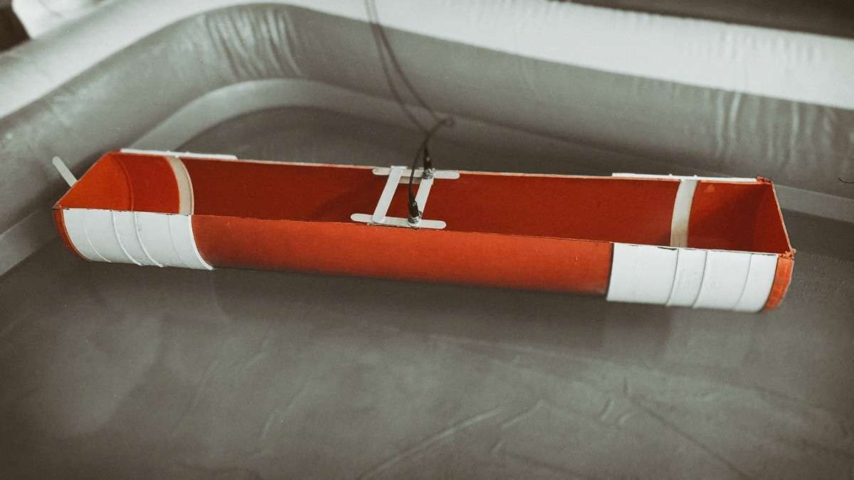
For comparing roll period measurements, I conducted a series of tests on a rigid system consisting of a PVC cylinder. The cylinder was sectioned longitudinally at 3/4 of the diameter. It was equipped with caps on both ends to enable buoyance, and immersed in a water-filled tank (see Figures 1 and 2).
Two IEPE accelerometers are appropriately positioned on the floating body to record the acceleration on the roll plane. IEPE accelerometers measure linear acceleration based on the piezoelectric effect. I used these to calculate linear accelerations along the vertical axis.
This setup ensured that the oscillation of the two instruments was out of phase. Each represents the effective vertical oscillation of the left or right side of the floating body. Although I could measure the floating body’s transverse acceleration (drift accelerations), such measurements were deemed less relevant for this study.
Measurement setup
For the measurements using IEPE accelerometers, I verified that the cables did not introduce any interference factors in our model. I secured the wires to the bottom to prevent them from hitting the hull and creating impulsive forces. Using a bracket, I supported their respective ends to ensure they did not act as a damping factor for roll motion - see Figures 2 and 3.
The additional masses used were rectangular steel bars with a 1.5 kg mass each. I arranged the bars to have their centers of mass aligned with the vertical axis passing through the model’s center of mass. I could approximate these masses as a distributed load that primarily affects the geometric properties of the system longitudinally rather than transversely.
This assumption allowed me to consider that the system’s moment of inertia remains substantially unchanged. The associated mathematical treatment then only takes the variation in mass into account.


I used an inflatable pool to submerge the floating model. I selected the pool size to have reflections and optimize the model arrangement.
In most tests, the reflection effects were negligible due to the pool walls’ partial absorption of wave motion. Using a goniometer, I established an initial "standard" condition with a roll angle of approximately ten degrees. I chose this value to minimize non-linear effects with potentially significant impact.
A goniometer is a device that permits the rotation of an object to a definite position.
After identifying the peaks x1 and xm+1, I calculated the logarithmic decrement. For each test, I obtained the value of δ. Operating conditions significantly influence the results and adopting an exact condition ‘standard’ is impossible. I used the arithmetic mean of these values to deduce the value of the dimensionless damping coefficient through the following relationship:


My professor provided the KRYPTON data acquisition system (DAQ). KRYPTON was applied to collect the data. The DewesoftX software platform performed all the required signal processing.


I worked with a basic setup. I used two input channels to connect two IEPE accelerometers simultaneously. The software visualized the voltage output signal over time. I plotted the vertical motion of the two accelerometers during the roll motion. I observed their behavior over time to acquire peak values and “manually” calculate control factors.
Accelerometer data analysis
I made a difference between the two accelerometer signals to obtain a configuration isolated as much as possible from offset and sensitivity errors. Offset errors refer to deviations of the accelerometer signal when not subjected to acceleration.
Each accelerometer can have a different offset. The offset represents a constant value added to or subtracted from the measured acceleration signal. By placing two accelerometers on separate sections, I could obtain offset measurements. I used those to compensate for and eliminate the effect of errors. Sensitivity errors refer to differences in the sensitivity response between accelerometers.
Each accelerometer can also have a different sensitivity. The sensitivity represents a conversion scale between the measured physical acceleration and the output electrical signal. By placing two accelerometers and comparing their respective measurements, any discrepancy in sensitivity is detectable, and I could calibrate the signals accordingly. To perform the calibration, I used the pseudocode available in the Math functionality, an informal programming description that does not require any strict programming language syntax.
I applied an IIR filter to isolate the frequency components of interest and accurately calculate the logarithmic decrements over a broader sequence of samples. An IIR filter has a low-pass filter of around 5 Hz. The filter preserves the main roll component at the natural frequency of 1 Hz and monitors the behavior of disturbance components - see Figure 5.

Once I set the IIR filter correctly, the signal is cleaned of impurities, offering better resolution (see Figure 6). Although the signal natural frequency was dominant initially, this was not the case towards the end of the experiment. Disturbance frequencies appeared in both tests.

I conducted the tests by applying an IIR filter and adding a distributed mass of three kg - see Figures 7 and 8. In these tests, slightly lower disturbance frequencies appeared and were more evenly distributed compared to the first test. There was significant persistence of noise and leakage in the frequency spectrum.

Mechanisms appeared sometime after the measurement started. They generated a temporary pseudo-overdamping extinguishing in a fraction of a second. This phenomenon further reduced the oscillation period until it almost ceased. Moments later resumed with the expected logarithmic behavior (see Figure 8).

I attribute the phenomenon to some frequency components around the octave of 2 Hz - see Figure 8. I explain it as a form of interaction between the roll and the waves reflected from the tank wall. Tables 1, 2, and 3 summarize the logarithmic decrement, damping, and roll period values considering only bodyweight tests.
| Test | δ[-] | ζ[-] | T[s] |
|---|---|---|---|
| 1 | 0.190 | 0.0302 | 0.95 |
| 2 | 0.220 | 0.0350 | 0.95 |
| 3 | 0.180 | 0.0286 | 0.95 |
| 4 | 0.190 | 0.0302 | 1.00 |
| Values | δ | ζ | T |
| Medium | 0.195 | 0.0310 | 0.96 |
Finally, I have two important considerations. The use of a very high sampling frequency did not benefit my measurements. A proficient user must always know what type of phenomenon to expect and its corresponding period.
I only needed to count the peaks with a simple counter and measure the amplitude value to obtain the logarithmic decrement.
Setting the sampling frequency from the beginning would have been better. The resulting graph demonstrates this - see Figure 9. It shows how undersampling at 40Hz significantly improved the signal quality - almost as well as using the IIR filter.

When I reduce the sampling frequency, I eliminate high-frequency components that may correspond to noise or unwanted interference. This reduction cleans the signal and makes the desired components, such as the 1-second roll period, more prominent.
Aliasing is a phenomenon where frequencies higher than half the sampling frequency (Nyquist frequency) fold back into the lower frequency range. This creates distortions in the signal. By reducing the sampling frequency, you reduce the amplitude of the frequency spectrum of high-frequency components, thereby reducing the possibility of aliasing.
Consider that downsampling results in a loss of high-frequency information. If there are components of interest in the signal beyond the reduced Nyquist frequency (20Hz in our case), they may be attenuated or completely lost during downsampling.
There is a considerable difference between the raw signal and the undersampled signal (see Figure 9). Finally, I conclude that, unlike the IIR filter, the FIR filter wasn’t helpful. A simple low-pass filter wasn’t sufficient, and it was necessary to resort to proportional integral derivative control within the IIR.
| Test | δ[-] | ζ[-] | T[s] |
|---|---|---|---|
| 1 | 0.163 | 0.0260 | 0.98 |
| 2 | 0.161 | 0.0257 | 1.01 |
| 3 | 0.151 | 0.0240 | 0.99 |
| Values | δ | ζ | T |
| Medium | 0.158 | 0.0252 | 0.99 |
| Medium | 0.195 | 0.0310 | 0.96 |
| Test | δ[-] | ζ[-] | T[s] |
|---|---|---|---|
| 1 | 0.169 | 0.0269 | 0.99 |
| 2 | 0.160 | 0.0254 | 0.99 |
| 3 | 0.171 | 0.0272 | 0.99 |
| 4 | 0.199 | 0.0316 | 0.96 |
| Values | δ | ζ | T |
| Medium | 0.175 | 0.028 | 0.98 |
Conclusion
In this study, I aimed to measure the roll period by taking three approaches:
One using two IEPE accelerometers.
Second by using a mathematical model.
A third one uses an Inertial Measurement Unit (IMU) - see Tables 1, 2, and 3.
The results obtained with these three approaches were similar concerning logarithmic decrement, dimensionless damping coefficient, and rolling period. They highlight the validity of the choices I made, which, although simplified, were correct from a mathematical and physical standpoint.
Measurements conducted through the IEPE accelerometers, the mathematical method, and the IMU system indicate that adding masses affects all variables. In the case of adding a weight of 3 kg, I observed phenomena related to constructive interference arising from the waves generated by the model’s motion and then reflected. The vibrations of the system's walls give rise to significant and evident periodic forces.
It is necessary to consider that the results are based on a simplified model and may not reflect the behavior of a more complex system. To fully understand the dynamics of such a system, further studies and analyses may be needed.