Go-Kart Chassis Modal Analysis: Experimental Testing and FEM Validation
Aljaž Luznar
University of Ljubljana
November 20, 2026
A go-kart chassis serves as both the structural frame and the primary suspension element, making its dynamic behavior critical to vehicle performance and durability. This study compares experimentally measured modal properties of a free-free kart chassis with the results of a custom finite element model developed from scratch in Python. The close agreement between measured and simulated natural frequencies demonstrates the model’s accuracy while highlighting the limitations of a single-axis experimental measurement setup.
Understanding the vibration behavior of a go-kart chassis is essential for structural durability and on-track performance. Unlike vehicles with conventional suspension systems, a go-kart relies on its tubular steel frame to provide the necessary flexibility and damping.
In this study, I performed an experimental modal analysis (EMA) of a bare go-kart chassis using a Dewesoft DEWE-43A data acquisition system and DewesoftX software. I then compared the measured natural frequencies and mode shapes with results from a custom finite element model (FEM) developed from scratch in Python.
The results show close agreement between the experimental measurements and numerical simulations, with most matched natural frequencies differing by less than 5%. The comparison also reveals the limitations of measuring vibration along a single axis.
Why go-kart chassis modal analysis matters
A go-kart chassis must balance two conflicting structural requirements. It needs enough flexibility to accommodate torsional and bending deformations, helping distribute loads evenly across all four wheels and maintain grip on the track. At the same time, it must be rigid enough to withstand operational loads.
The chassis's dynamic response therefore directly affects mechanical grip, handling, stability, and ultimately, lap times.
During operation, the track surface roughness and the powertrain impose dynamic loads on the chassis. The kart in my analysis has a Rotax 125 Junior MAX Evo engine: a single-cylinder, two-stroke engine with a 125 cm³ displacement that produces 23 horsepower at 8,500 RPM.
The engine generates harmonic excitation at frequencies that depend on its rotational speed. The fundamental excitation frequency corresponds to the first engine order and is calculated as f = RPM / 60, with additional harmonics occurring at higher orders.
At the maximum engine speed of approximately 14,000 RPM, the fundamental excitation frequency reaches 233 Hz. To capture the second-order harmonics, I extended the modal analysis frequency range to 470 Hz.
When any of these operational excitation frequencies coincides with a natural frequency of the chassis, resonance occurs. Under resonant conditions, vibration amplitudes rapidly escalate and are limited only by the light material and the frame's structural damping.
Under the rules of the Fédération Internationale de l'Automobile (FIA), racing kart geometry is strictly standardized, leaving very tight margins for modifications. The frame is constructed from chromium-molybdenum steel (25CrMo4 / 1.7218) tubes of varying diameters, with a uniform wall thickness of 2 mm. Figure 1 shows the fully equipped kart with the Rotax 125 Junior MAX Evo engine, while Figure 2 presents the bare chassis utilized for the modal analysis.


Fundamentals of experimental and numerical modal analysis
Experimental modal analysis determines how the physical chassis vibrates by measuring its response to controlled excitation. Numerical modal analysis predicts the same behavior using a mathematical model of the structure. Comparing the two methods makes it possible to evaluate how accurately the Python-based finite element model represents the real chassis.
How experimental modal analysis works
Experimental modal analysis is a procedure for identifying a structure's dynamic properties from its measured response to a known excitation. These dynamic properties are the natural frequencies, damping ratios, and mode shapes, which together form the structure's modal model. The structure is assumed to behave in a linear, time-invariant manner so that I can describe its behavior independently of the particular excitation applied.
The quantity that links the input force to the measured response is the Frequency Response Function. In modal testing, engineers most often measure the response with an accelerometer, so the relevant form of the Frequency Response Function is the accelerance, which relates the acceleration response to the input force in the frequency domain. It takes the form:
The accelerance is a complex function of frequency and therefore has both magnitude and phase. A natural frequency appears as a sharp peak in the accelerance magnitude, accompanied by a phase shift of about 180 degrees.
A single Frequency Response Function locates the natural frequencies but does not describe how the structure deforms at each. To recover this information, I must measure the Frequency Response Function at many points distributed over the structure, and several measurement strategies exist. The relative amplitude and phase of the response at every point of the grid, evaluated at a given natural frequency, define the corresponding mode shape.
Several methods are available for acquiring these Frequency Response Functions. In the roving hammer method, a single accelerometer, fixed at a reference point, measures the response. In contrast, the excitation point is moved across the grid with the hammer from one measurement to the next, yielding one row of the receptance matrix. In the complementary roving accelerometer method, you hold the excitation point fixed and move the accelerometer across the grid, yielding one column of the receptance matrix rather than one row.
When more measurement channels are available, you can perform the test with one excitation point and many simultaneous response sensors (a single-input multiple-output configuration) or with several simultaneous excitation points and many response sensors (a multiple-input multiple-output configuration). Because of the structure's reciprocity, a single row or column of the receptance matrix is sufficient to reconstruct the mode shapes.
Finite element modal analysis using beam elements
I built the numerical model with three-dimensional beam finite elements based on the classical Euler-Bernoulli beam theory. This theory assumes that plane cross sections remain plane and perpendicular to the deformed neutral axis, thereby neglecting shear deformation and also neglecting the rotary inertia of the cross-section in bending. This method provides an accurate approximation for slender members such as the tubes of a kart chassis.
Each element connects two nodes, and each node has six degrees of freedom: three translations and three rotations. The element, therefore, has twelve degrees of freedom in total. With this set of degrees of freedom, a single element captures four independent deformation mechanisms. These are axial extension along the beam axis, torsion about the beam axis, and bending in each of the two planes containing the beam axis.
I can assemble the element stiffness matrix and the consistent mass matrix from the contributions of these four mechanisms, and both are 12×12. The mass matrix is consistent because I derive it from the same interpolation functions as the stiffness matrix, rather than by lumping mass at the nodes.
| Mechanism | DOF |
|---|---|
| Axial extension along x | 𝑢1, 𝑢2 |
| Torsion about x | 𝜃𝑥1, 𝜃𝑥2 |
| Bending in the xy plane | 𝑣1, 𝜃𝑧1, 𝑣2, 𝜃𝑧2 |
| Bending in the xz plane | 𝑤1, 𝜃𝑦1, 𝑤2, 𝜃𝑦2 |
Because the chassis tubes have circular cross sections, the formulation simplifies. The two principal second moments of area are equal due to the section's symmetry, and the torsion constant of a circular section equals its polar second moment of area, which in turn equals twice the bending second moment of area. A circular section also does not warp under torsion, so the cross sections remain plane and rotate about the beam axis.
I first form the element matrices in a local coordinate system attached to the element, and then rotate them into the common global coordinate system before forming the global system matrices. Three-dimensional rotation requires a reference vector to fix the cross-section's orientation in the plane perpendicular to the beam axis, because the two end nodes define only the direction of the beam axis. For a circular section, the element matrices are rotationally symmetric about the beam axis, so the assembled global matrices do not depend on the particular choice of reference vector. However, I still must supply a valid reference vector for the computation to proceed.
The global stiffness and mass matrices are assembled from the transformed element contributions and define the undamped free-vibration equation. I obtain the natural frequencies and mode shapes by solving the generalized eigenvalue problem:
Each eigenvalue gives a natural frequency ω, and each eigenvector gives the associated mode shape 𝜑.
Experimental and numerical modal analysis methods
Go-kart chassis modal testing with Dewesoft
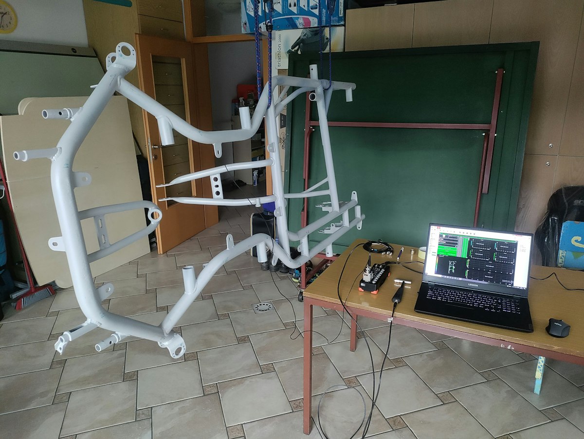
I tested the chassis under free-free boundary conditions. By suspending the chassis from a single stretchable elastic cord, as shown in Figure 3, I realized this condition. I chose a free-free condition because it is the easiest boundary condition to reproduce accurately in both practice and the numerical model, and it is highly repeatable.


Only two DSI-ACC adapters were available for the DEWE-43A data acquisition system. I used one for the modal hammer and the other for a single accelerometer axis.
Because the modal hammer had to remain connected throughout the test, only one channel was available to measure the chassis response. The experimental modal analysis therefore used a single-input single-output (SISO) configuration, recording one excitation signal and one response signal at a time.
I selected the roving hammer strategy over the roving accelerometer strategy for three reasons. The first reason is reciprocity. The receptance matrix of a linear structure is symmetric according to the Maxwell-Betti theorem, so measuring one row is equivalent to measuring one column, and no modal information is lost. A single row is therefore sufficient to reconstruct the mode shapes.
The second reason is constant mass loading. The accelerometer adds a small mass to the structure at its mounting point, and keeping it fixed ensures this added mass always acts at the same known location. In a roving accelerometer test, the added mass would move from point to point and slightly alter the structure at each measurement, making comparison with the numerical model less clear. The third reason is speed and repeatability.
Once the accelerometer is mounted, the adapters and the sensor are not touched again during a measurement series; only the hammer is moved from point to point. This removes a source of variation between the individual measurements.
The accelerometer and the excitation were both oriented normal to the ground when the kart is in its normal operating position. I chose this direction because the chassis is least stiff in this direction, so most of the mode shapes are expected to exhibit their largest deformations along it. Figure 4 shows the accelerometer orientation and the excitation direction.


Figure 5 shows the measurement chain, which consists of these components:
1x Dewesoft DEWE-43A USB data acquisition system.
DewesoftX software with the Modal Test and the Modal Analysis modules.
1x instrumented modal hammer, connected to the DEWE-43A through a DSI-ACC adapter, used to apply and measure the excitation force.
1x uniaxial IEPE accelerometer, connected to the DEWE-43A through a DSI-ACC adapter, used to measure the response and mounted with its sensitive axis oriented vertically.

I first marked the measurement points directly on the chassis, approximately evenly distributed over the whole structure, as shown in Figure 6. Marking the points on the physical structure ensured that I struck each point at the same location each time I repeated a measurement. I then reproduced the same set of points in the DewesoftX geometry editor, connecting them with lines representing the tubes to improve visualization of the structure and the measured mode shapes.

In the Modal Test module, I configured the impact hammer acquisition. A trigger on the force channel, together with a small pre-trigger, reliably captured each impact. Because a lightly damped steel structure continues to vibrate long after each impact, I applied an exponential window to the response to reduce leakage.
I set the sampling rate to 2000 Hz, which places the Nyquist frequency at 1000 Hz. This setting covers the excitation range identified in the previous section and lies well above the highest measured natural frequency. I computed the spectrum with 12000 spectral lines, which gives a frequency resolution of 0,083 Hz and a block length of 12 s. I kept a pause longer than the block length between successive impacts, so each block captured the full decay of the response before the next impact.
The choice of hammer tip affects the quality and frequency range of the excitation. I selected a semi-hard ceramic tip because it produced a sufficiently wide excitation spectrum. A rubber tip did not excite a wide enough frequency band, while a steel tip caused frequent double hits that required repeated measurements.
At each measurement point, I performed four impacts and averaged the results to improve signal quality and reduce noise and variations between individual impacts. Figure 7 shows the signals monitored during the modal test.


After measuring all the points, I processed the recorded Frequency Response Functions in the Modal Analysis module. I added all transfer functions to the analysis over the 0-470 Hz band, and used a stabilization diagram to separate physical resonances from purely numerical poles. I selected stable poles that were consistent in both frequency and damping on the stabilization diagram, then computed the modal parameters from this selection.
Building a go-kart chassis FEM model in python
I developed the go-kart chassis finite element model (FEM) from scratch in Python, following the beam theory described above.
The modeling process began with defining the chassis geometry and tube cross sections. I then calculated the element stiffness and mass matrices, transformed them into the global coordinate system, and refined the mesh. Finally, I assembled the global matrices, adjusted the model's mass to match the measured chassis, applied free-free boundary conditions, and solved the eigenvalue problem to obtain the natural frequencies and mode shapes.
Rather than entering it by hand, I took the chassis geometry from a CAD model. The geometry consists of nodes with three-dimensional coordinates and a list of elements connecting them, each representing a frame tube. The base geometry consists of 29 nodes and 34 tube segments. I modeled the two elements connecting node 28 to reflect the actual geometry; however, I hid them from the animations for clarity and to allow a more intuitive comparison with the experimental measurements.
Figure 8 visualizes this geometry, together with the node numbering.


The steel frame has a Young's modulus of 210 GPa, a density of 7850 kg/m³, and a Poisson ratio of 0.3. I computed the shear modulus I needed for the torsional stiffness from Young's modulus and the Poisson ratio. Each tube has its own outer diameter, ranging from 13 mm to 32 mm across the frame, with a uniform wall thickness of 2 mm. From these dimensions, I computed the cross-sectional area and second moment of area for each tube as a hollow circular section.
For every element, I formed a twelve-by-twelve local stiffness matrix and a twelve-by-twelve consistent mass matrix. I set the torsion constant of each circular tube equal to twice its second moment of area. I first expressed both matrices in the element's local coordinate system and then rotated them into the global coordinate system using a transformation matrix. This transformation matrix is block diagonal and consists of a single three-by-three rotation matrix repeated for the element's two translations and two rotations.
The line that joins its two end nodes defines each element’s local x-axis, while a reference vector fixes the orientation of the local y and z axes. The program selects this reference vector automatically. It first tries the global vertical direction because most tubes lie close to the horizontal plane and are therefore rarely parallel to it. It falls back to another global axis whenever a tube is parallel to the first choice. As explained in the theory, the circular cross-section makes the result independent of the particular reference vector, so this automatic choice does not affect the computed frequencies.
Each tube in the base geometry is subdivided into several shorter finite elements to ensure the mesh is fine enough to represent the mode shapes accurately. A target element length controls the subdivision. I divide each tube into equal segments to bring the element length as close as possible to this target, and I represent at least one element for each tube. The cross-section of a tube is inherited by all elements, so the refined model retains the same physical properties as the base geometry. Figure 9 shows the meshed structure.


The bare beam frame is lighter than the real chassis because the real chassis includes welds and details that I cannot model with beam elements. To account for this difference, I added concentrated point masses at the translational degrees of freedom of the nodes where the hardware is attached. I then distributed the remaining difference, up to the measured mass of 12.6 kg, uniformly among all nodes. I added only the translational inertia of these point masses and neglected their rotational inertia. After this step, the model's total mass matches the chassis's measured mass.
I analyzed the chassis under the same free-free condition as in the experiment to avoid constraining degrees of freedom and to use the global matrices directly. By solving the generalized symmetric eigenvalue problem for the global stiffness and mass matrices, I obtained the natural frequencies and the mode shapes.
Modal analysis results and FEM validation
FEM mesh convergence and model accuracy
I analyzed the chassis under free-free conditions, so the first six natural frequencies are rigid-body modes with frequencies of approximately zero. These six modes do not represent elastic deformation; therefore, I excluded them from the results. The remaining elastic modes are numbered from 1 onward throughout this report, making them easier to compare with the modes identified in the experiment. I then verified the convergence of the numerical model by repeating the entire analysis at four mesh densities obtained by progressively reducing the target element length, each containing 127, 259, 508, and 1024 elements. This allowed me to verify the convergence of all elastic natural frequencies within the analyzed band. For clarity, Table 2 reports five representative modes distributed across the band rather than the full set.
I selected the finest mesh (1024 elements) as the reference solution and computed each coarser mesh's deviation relative to it. A small deviation, therefore, indicates that the frequency obtained on a coarser mesh is already close to the converged value.
Even with the coarsest mesh of 127 elements, all five representative natural frequencies in Table 2 differ from the converged values by approximately 0.1% or less. Further mesh refinement reduces these differences to negligible levels, confirming that the numerical results are effectively independent of mesh density.
Because the coarsest mesh already provides sufficient accuracy, I used it for the subsequent comparisons with experimental measurements and the mode-shape animations.
| Mode | Converged Frequency at 1024 elements [Hz] | Deviation at 508 elements [%] | Deviation at 259 elements [%] | Deviation at 127 elements [%] |
|---|---|---|---|---|
| 1 | 41,77 | +0,000 | −0,013 | −0,016 |
| 6 | 135,44 | −0,002 | −0,012 | −0,025 |
| 11 | 198,25 | −0,006 | −0,011 | −0,041 |
| 17 | 383,64 | −0,014 | −0,043 | −0,106 |
| 23 | 457,04 | −0,012 | −0,017 | −0,038 |
Measured natural frequencies and damping ratios
I extracted the modal parameters from the measured Frequency Response Functions in the Modal Analysis module by selecting the stable poles on the stabilization diagram (see Figure 10). Between about 41 Hz and 446 Hz, which covers the whole excitation range of interest, I identified twenty-seven modes.


The chassis is very lightly damped. The identified damping ratios range from about 0.02% to 0.24%, which is typical for a welded steel tube frame. The Modal Complexity Factor, which measures how far a mode departs from a real normal mode, remains low for nearly all modes, confirming good identification quality. Only two modes show a noticeably higher Modal Complexity Factor, suggesting these modes are more complex and more strongly coupled with their neighbors. Because the damping is so low, the measured damped frequencies are practically equal to the undamped natural frequencies and can be compared directly with the numerical results. Table 3 gives the complete set of identified modal parameters.
| Mode | Frequency [Hz] | Damping ratio [%] | MCF [%] |
|---|---|---|---|
| 1 | 41,50 | 0,102 | 3,25 |
| 2 | 43,12 | 0,096 | 0,33 |
| 3 | 84,44 | 0,068 | 0,46 |
| 4 | 89,58 | 0,092 | 0,38 |
| 5 | 133,26 | 0,039 | 1,05 |
| 6 | 144,95 | 0,041 | 0,21 |
| 7 | 154,21 | 0,025 | 0,38 |
| 8 | 160,32 | 0,032 | 0,58 |
| 9 | 172,94 | 0,031 | 0,29 |
| 10 | 179,40 | 0,047 | 0,28 |
| 11 | 188,71 | 0,240 | 1,26 |
| 12 | 194,62 | 0,064 | 5,18 |
| 13 | 218,27 | 0,088 | 1,05 |
| 14 | 229,78 | 0,094 | 0,33 |
| 15 | 234,37 | 0,122 | 0,48 |
| 16 | 270,12 | 0,085 | 1,16 |
| 17 | 287,49 | 0,069 | 0,83 |
| 18 | 298,48 | 0,022 | 0,46 |
| 19 | 320,02 | 0,076 | 0,19 |
| 20 | 359,74 | 0,039 | 6,85 |
| 21 | 368,16 | 0,043 | 0,25 |
| 22 | 371,89 | 0,035 | 0,18 |
| 23 | 388,30 | 0,035 | 1,46 |
| 25 | 402,61 | 0,076 | 2,94 |
| 24 | 410,37 | 0,052 | 2,33 |
| 26 | 427,95 | 0,048 | 0,35 |
| 27 | 445,56 | 0,031 | 2,99 |
Comparing experimental and FEM natural frequencies and mode shapes
I compare the experimental and numerical modes individually. I pair the modes by shape rather than by frequency order, because closely spaced modes can appear in different orders in the two sets. I give the frequency difference as the numerical value relative to the experimental value.
Because the measurement uses a single vertical axis, two consequences appear throughout. Several numerical modes move almost entirely in the horizontal xz plane of the chassis, so the vertical measurement axis could neither excite nor sense them, and they appear without an experimental counterpart. I could only match several pairs after reducing the numerical mode shape to its vertical component, since the measurement records only vertical motion. In contrast, the numerical mode shape is fully three-dimensional.
For the modes I could pair, the frequencies agree closely. Most pairs agree to within about 2%, and almost all of them agree to within about 4%. The only clearly larger difference is the first bending mode. A few mode-shape animations are shown, while all comparisons are presented in Table 4.
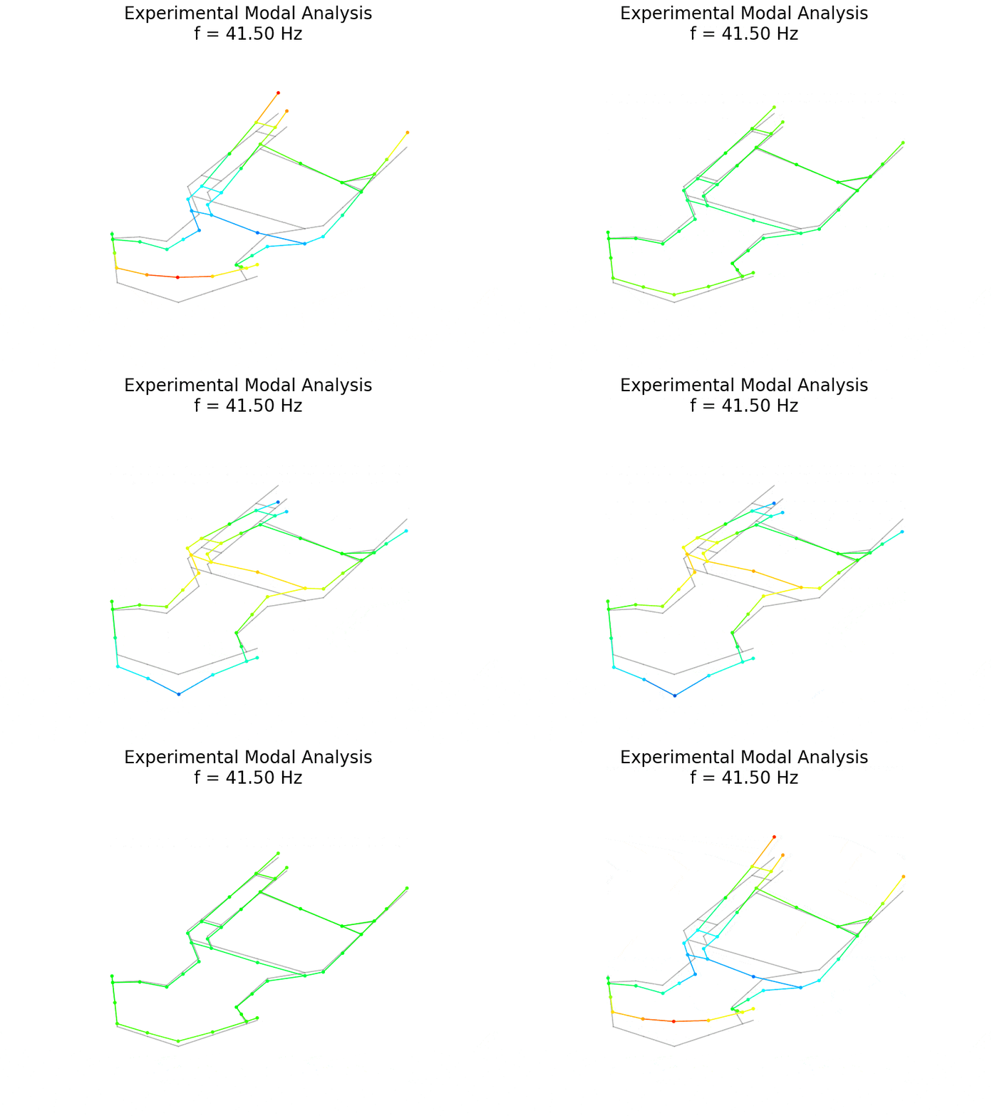
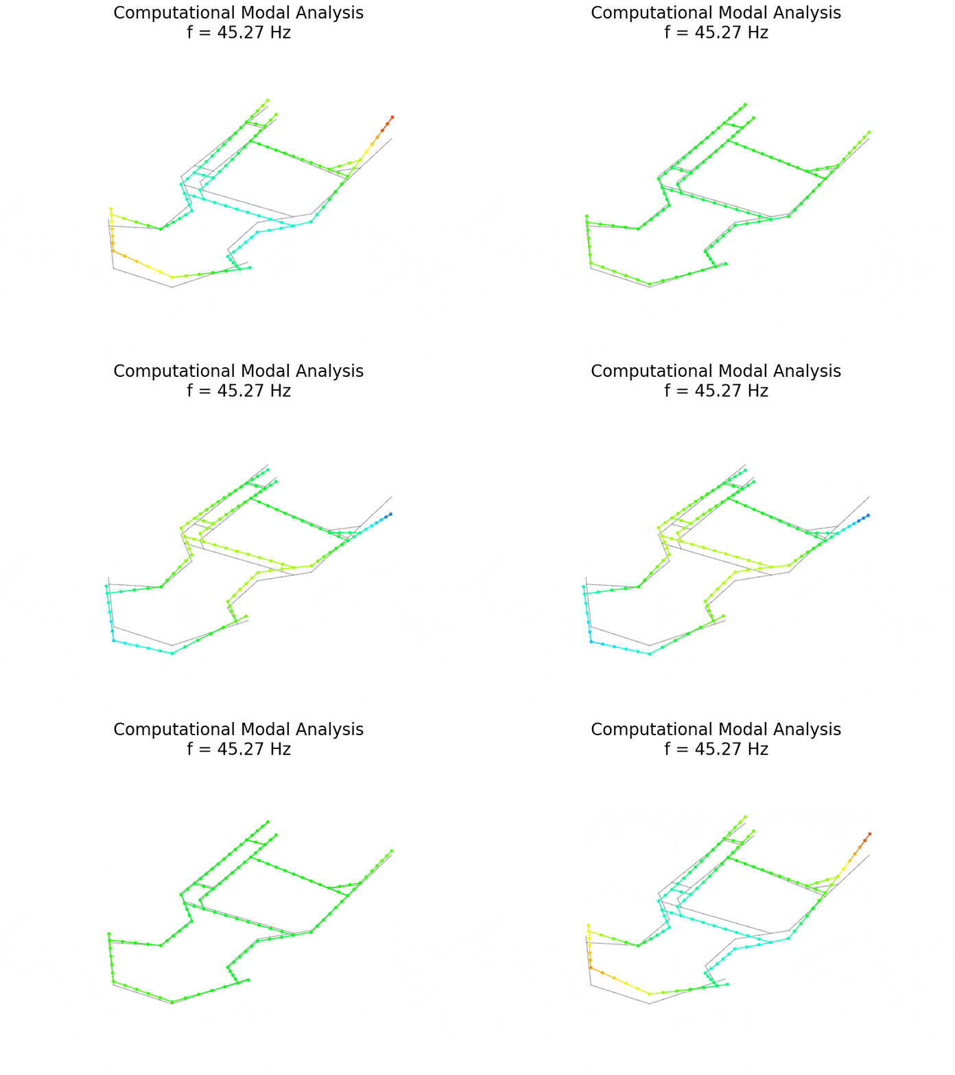
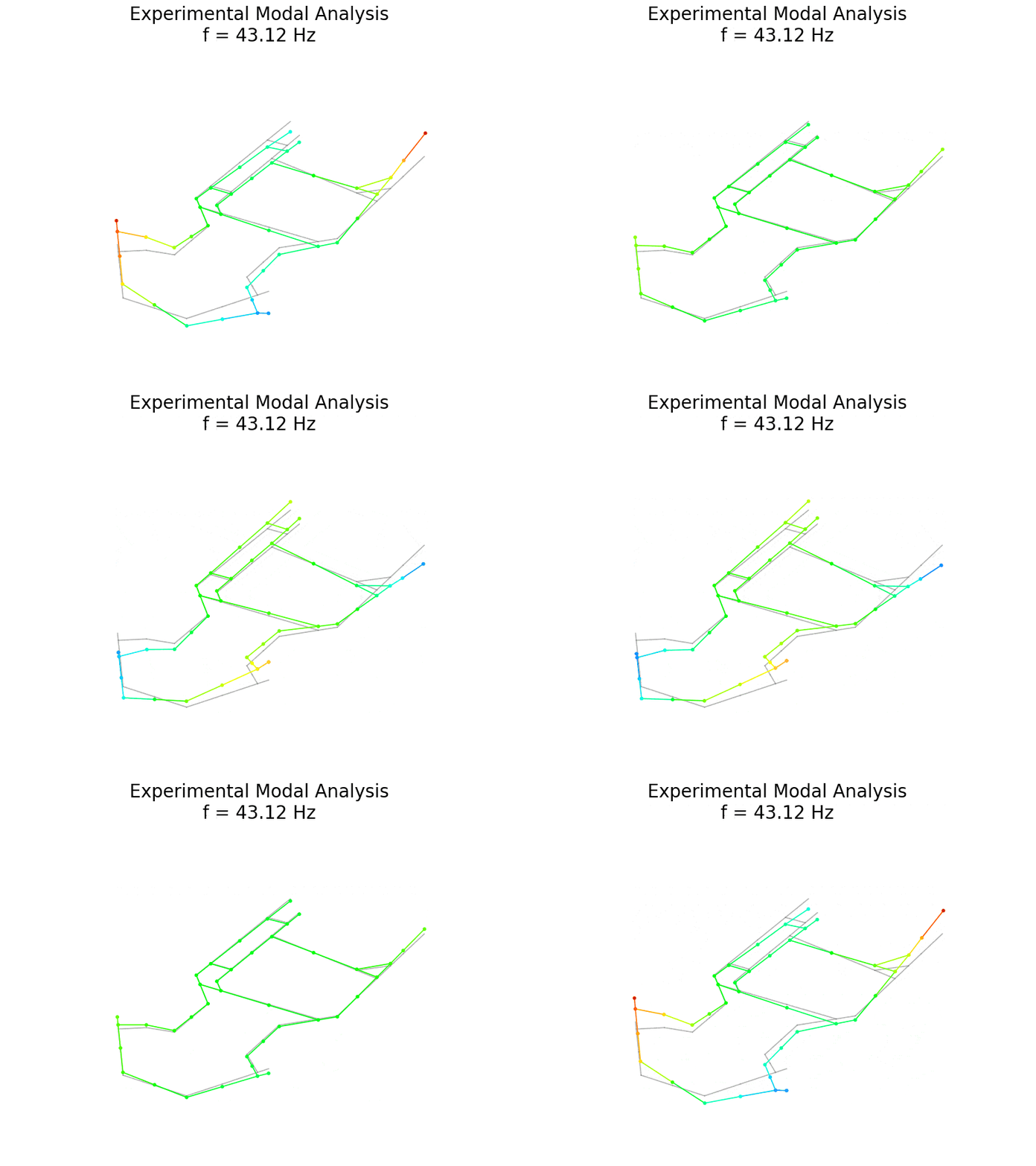
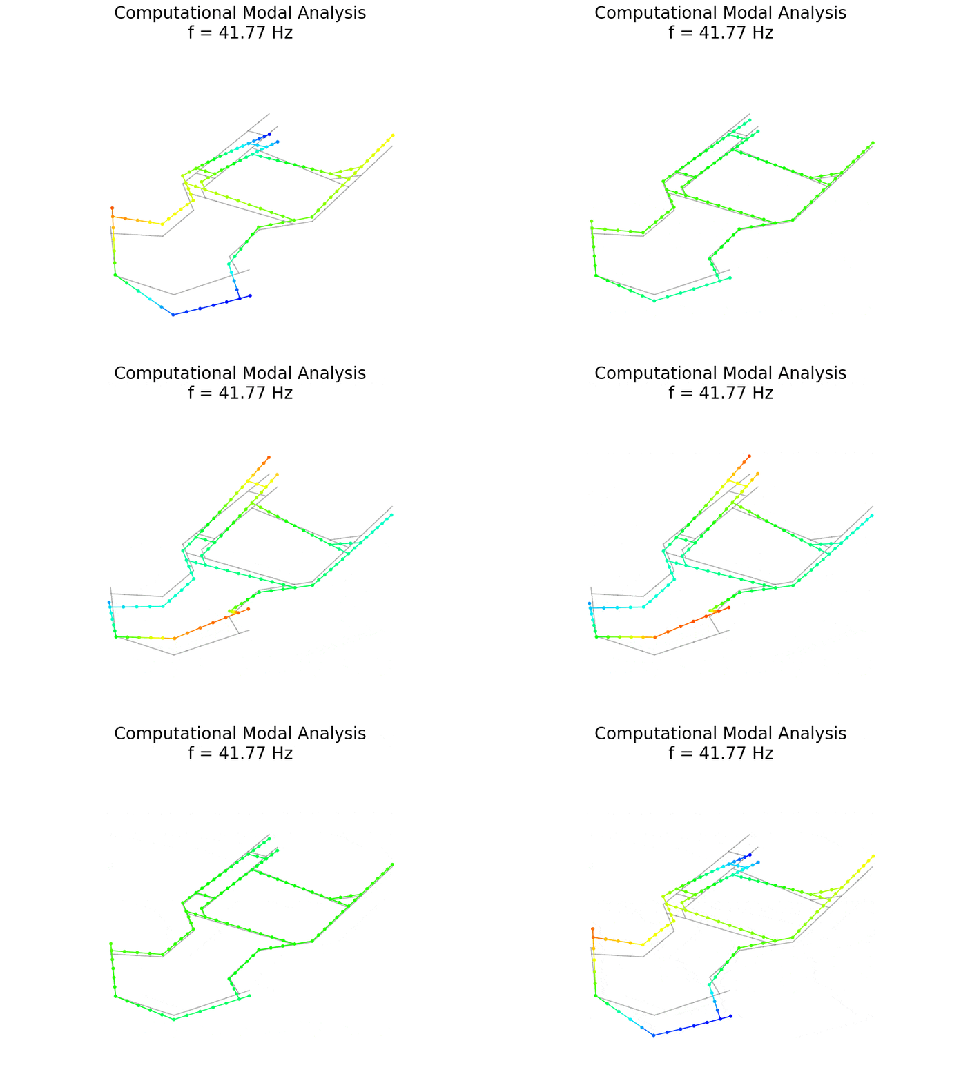
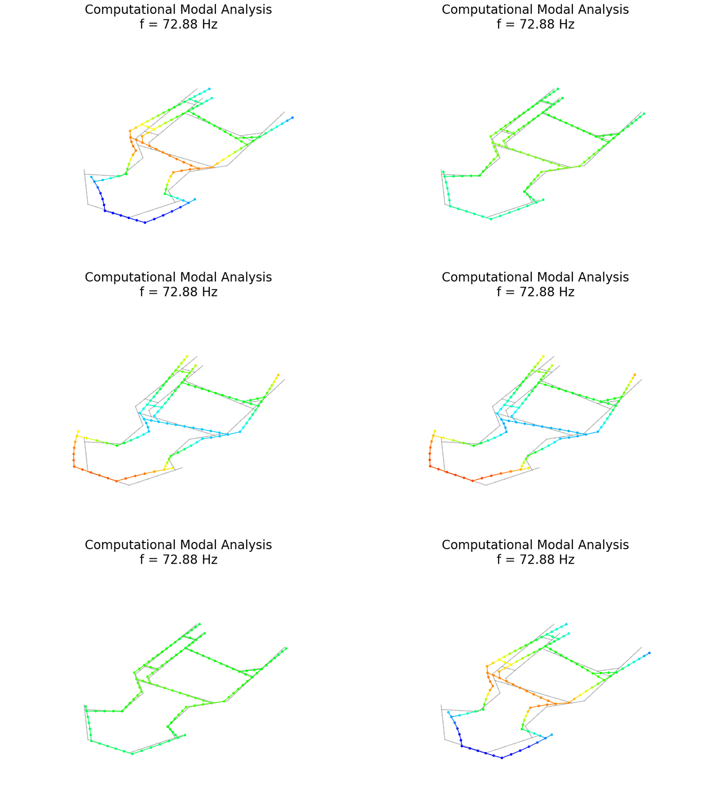
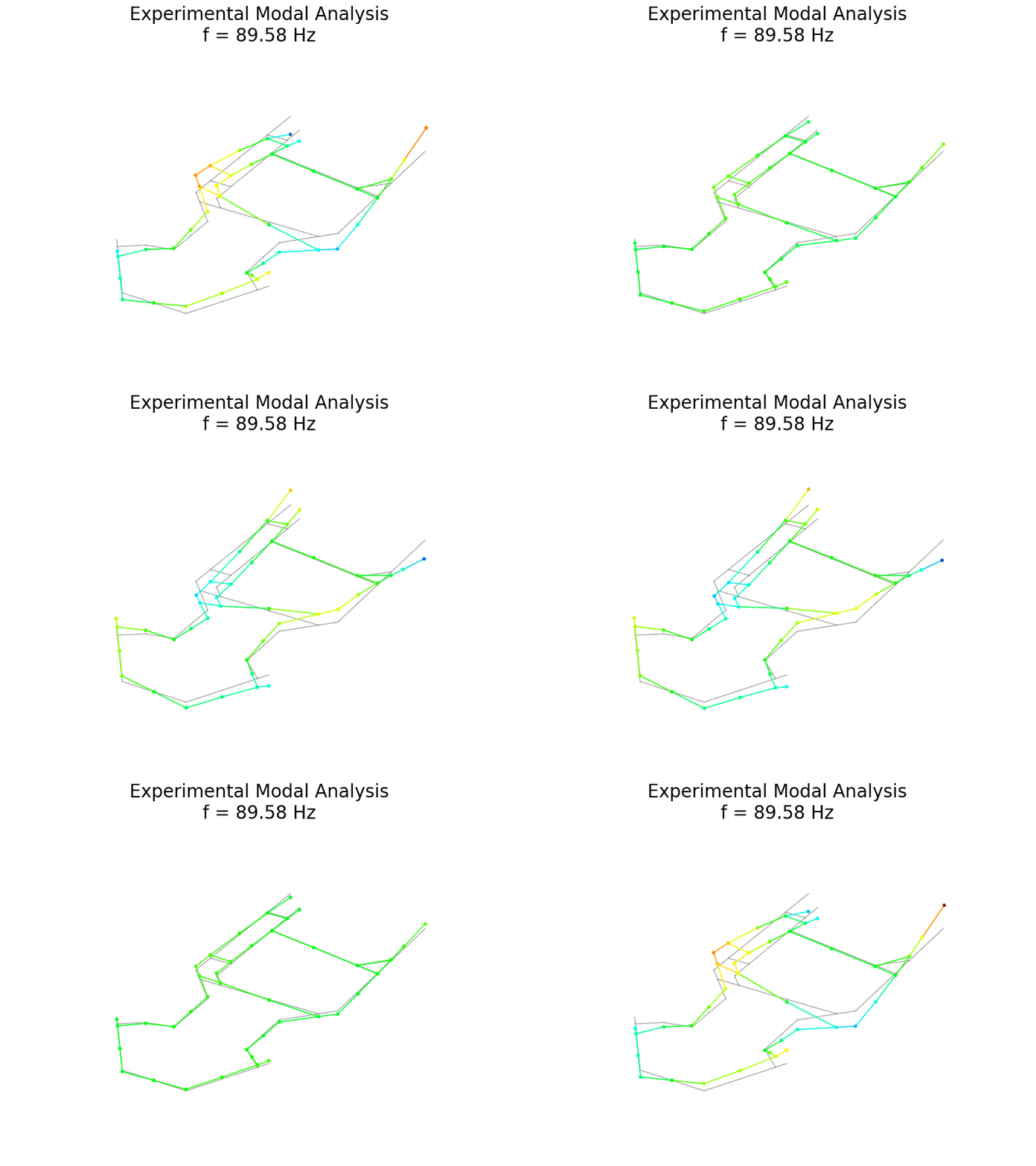
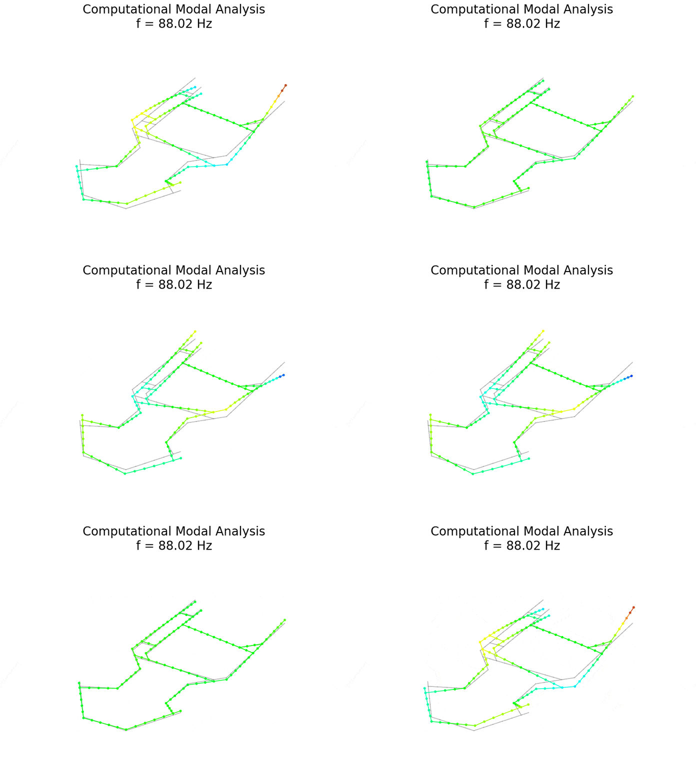
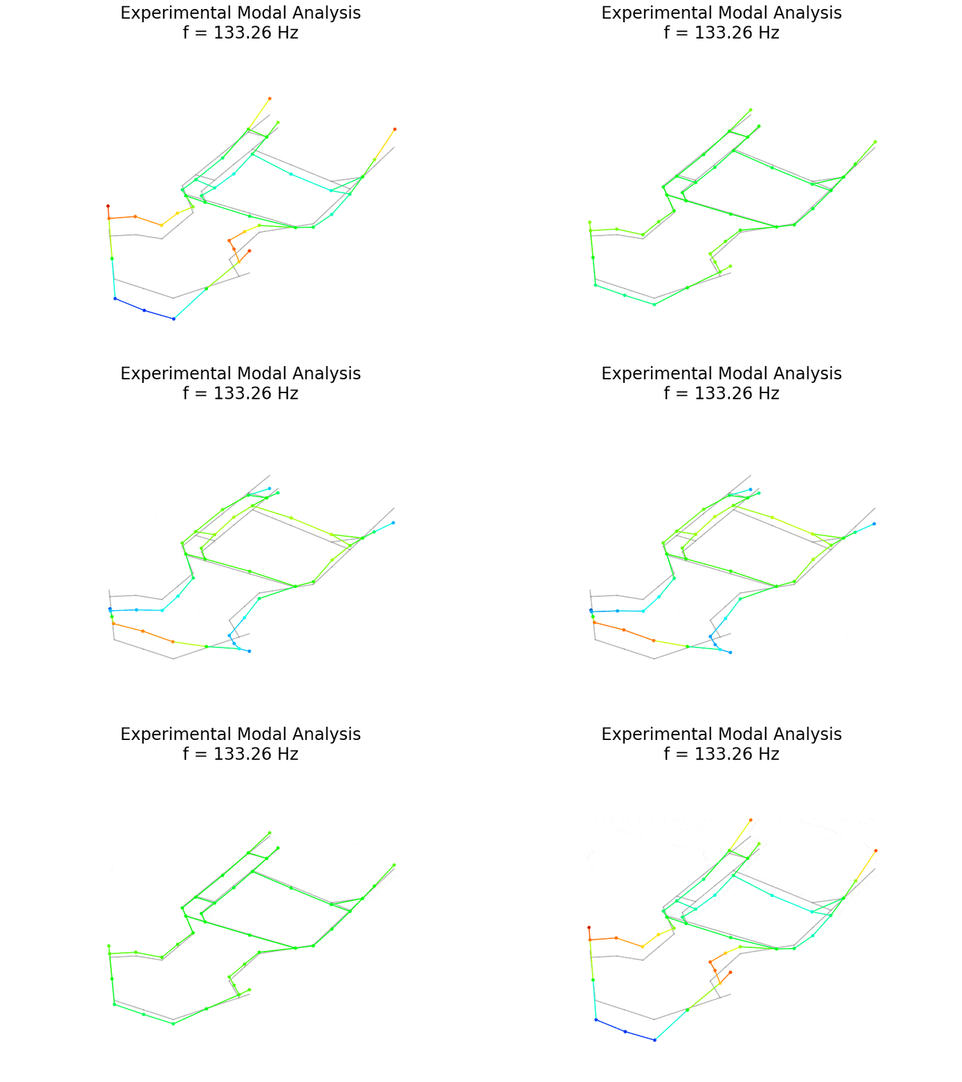
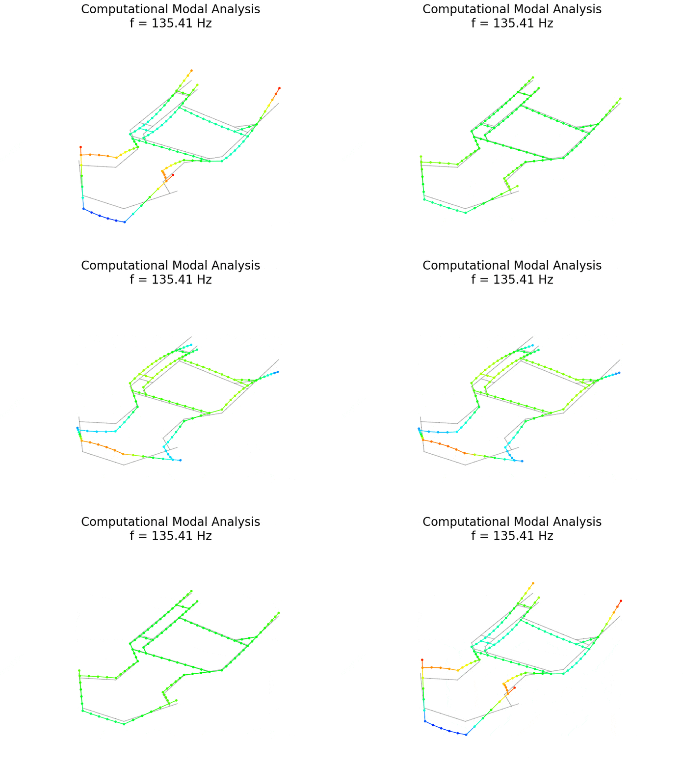
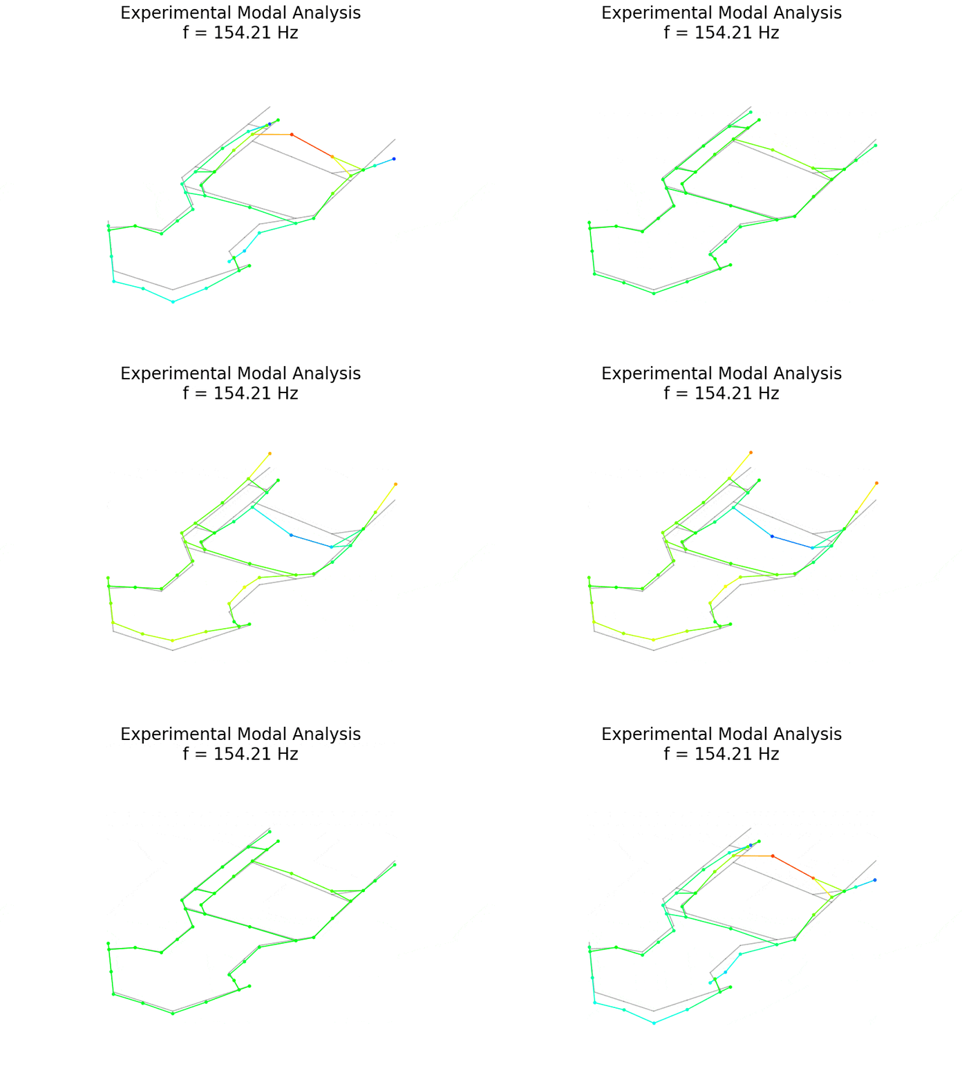
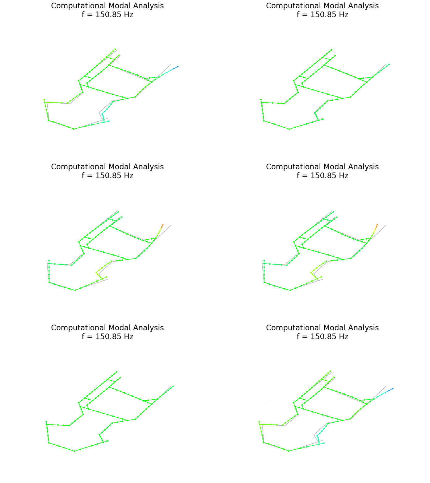
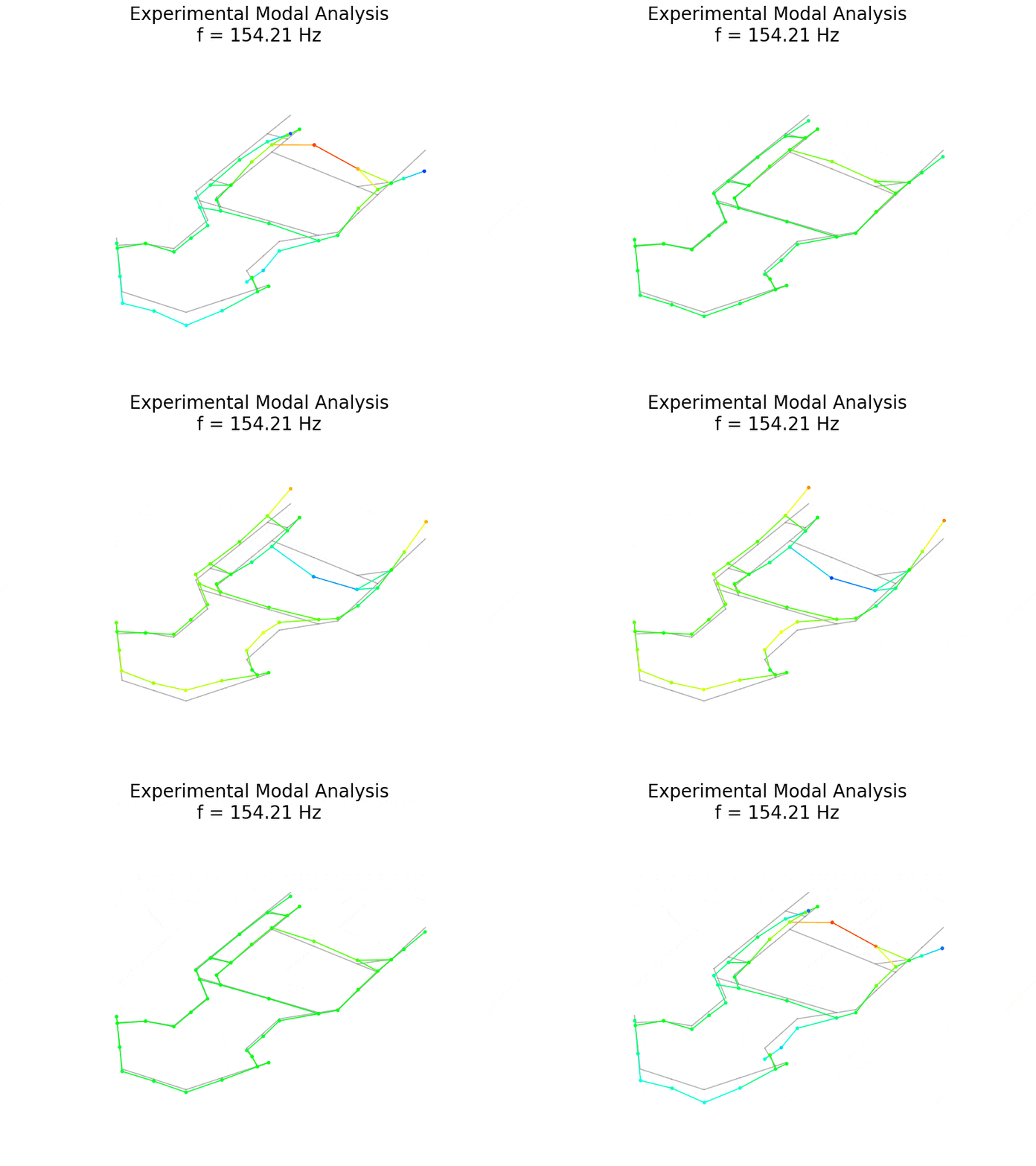
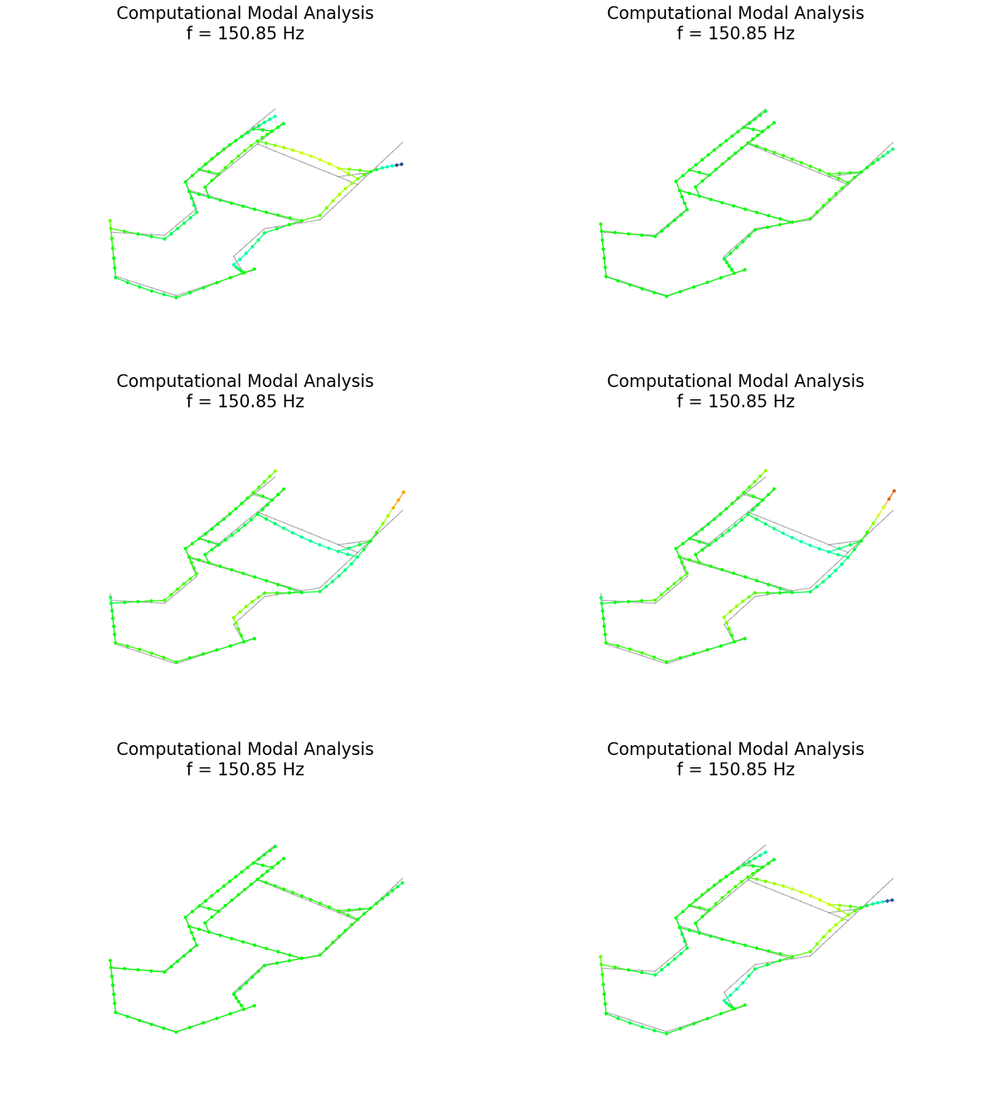
The following figures do not show the vertical component of the numerical shape.
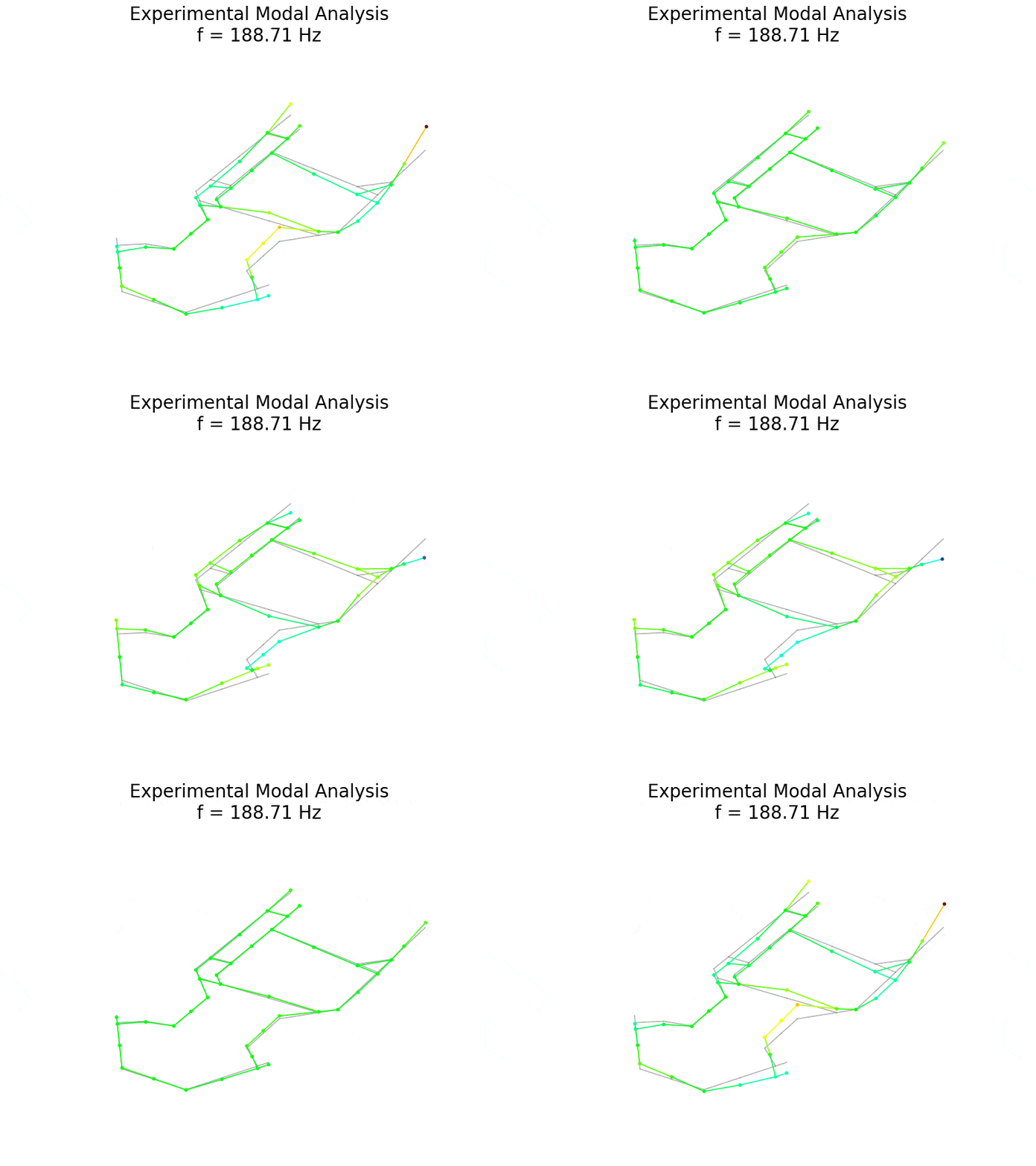
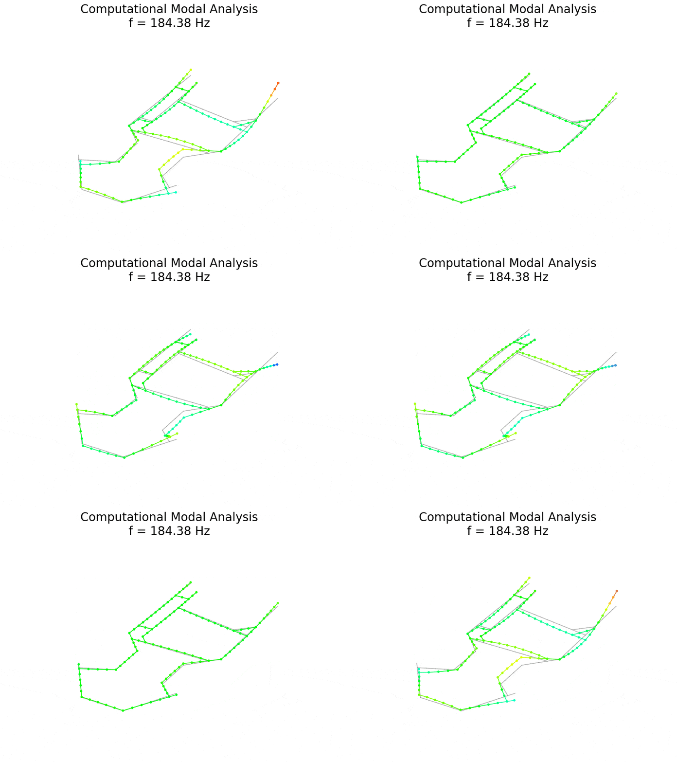
| Experimental mode | Experimental mode frequency [Hz | Computational mode frequency [Hz] | Difference [%] | Mode shape alignment |
|---|---|---|---|---|
| 1 | 41,50 | 45,27 | 9,1 | Fair |
| 2 | 43,12 | 41,77 | 3,1 | Fair |
| 72,88 | No experimental counterpart | |||
| 3 | 84,44 | No computational counterpart | ||
| 4 | 89,58 | 88,2 | 1,7 | Very good |
| 103,97 | No experimental counterpart | |||
| 5 | 133,26 | 135,41 | 1,6 | Very good |
| 6 | 144,95 | No computational counterpart | ||
| 7 | 154,21 | 150,85 | 2,1 | Good in vertical component |
| 8 | 160,32 | 160,09 | 0,1 | Fair in vertical component |
| 9 | 172,94 | No computational counterpart | ||
| 10 | 179,40 | 179,12 | 0,1 | Fair in vertical component |
| 11 | 188,71 | 184,38 | 2,2 | Very good |
| 12 | 194,62 | 198,17 | 1,9 | Very good |
| 211,72 | No experimental counterpart | |||
| 13 | 218,27 | 222,27 | 1,8 | Fair |
| 14 | 229,78 | No computational counterpart | ||
| 15 | 234,37 | No computational counterpart | ||
| 16 | 270,12 | 265,76 | 1,6 | Good |
| 279,86 | No experimental counterpart | |||
| 17 | 287,49 | No computational counterpart | ||
| 18 | 298,48 | No computational counterpart | ||
| 19 | 320,02 | 326,05 | 1,9 | Good |
| 20 | 359,74 | No computational counterpart | ||
| 21 | 368,16 | 383,23 | 4,2 | Fair in vertical component |
| 22 | 371,89 | 385,69 | 3,7 | Good |
| 23 | 388,30 | No computational counterpart | ||
| 25 | 402,61 | No computational counterpart | ||
| 24 | 410,37 | 420,55 | 2,5 | Good |
| 26 | 427,95 | 440,55 | 3,0 | Fair |
| 27 | 445,56 | 444,43 | 0,2 | Good |
Discussion: model accuracy and measurement limitations
Across the analyzed band from 41 Hz to 446 Hz, the custom Python beam model reproduces the chassis's dynamic behavior well for every mode that the single vertical measurement axis can observe. Wherever I could pair a mode, the natural frequencies agree within a few percent, and the shapes agree from fair to very good. This alignment is a strong result for an independently written model.
The remaining differences all have clear physical explanations. The first explanation concerns the two lowest modes, which form a closely spaced bending-torsion pair near 41-45 Hz. Their order swaps between the experiment and the model, and the model's bending mode is about 9% too high. When two modes lie so close together, small differences in the modeled stiffness of the welded joints, in the mass distribution, and in the small geometric asymmetries of the real frame are enough to change which mode comes first.
The second explanation concerns the single vertical measurement axis. Both the excitation and the response act only vertically, so modes that move mainly in the chassis's horizontal plane carry almost no vertical motion and cannot be observed. The same limitation explains why several pairs agree only when comparing the vertical component of the numerical shape, since the measurement observes only the vertical component of a fully three-dimensional motion.
The third explanation concerns the model's idealizations. Ideal circular beams represent the frame; the attached brackets and carriers are point masses with no rotational inertia; and the welds are unmodeled. The experimental modes with no numerical counterpart are most likely local modes of the attached hardware or modes shaped by these real features, none of which the idealized beam model can reproduce.
The two modes with the highest Modal Complexity Factor fall among those where matching is most difficult, consistent with this interpretation.
The fourth explanation concerns damping. The numerical model is undamped, so it predicts only natural frequencies and mode shapes and cannot reproduce the measured damping ratios. The measured damping is very low, below about 0.25%, as expected for a welded steel frame, and thus the undamped model is an appropriate idealization for predicting the frequencies and shapes.
These findings also have practical value for go-kart chassis design and optimization. The validated finite element model provides a fast, inexpensive way to predict how structural modifications affect the chassis's natural frequencies.
By comparing these frequencies with engine excitation, engineers can identify the engine speeds at which resonance may occur. Keeping modes with significant vertical motion away from frequently used engine excitation frequencies can help maintain consistent tire loads, preserve mechanical grip, reduce chassis chatter, and limit vibration-induced driver fatigue and component wear.
Conclusion: validating the go-kart chassis FEM model
This study combined experimental modal analysis of a go-kart chassis with a custom three-dimensional finite element model developed from scratch in Python. The two approaches were compared across a wide frequency range to evaluate the accuracy of the numerical model.
For most matched vibration modes, the simulated natural frequencies differed from the experimental measurements by less than 5%, while the mode shapes showed fair to very good agreement. The main exception was the first bending mode, with a frequency difference of approximately 9%. Overall, the results support the validity of the numerical model while identifying areas for further improvement.
The comparison is also valuable when it disagrees, because each disagreement has a clear cause. The two lowest modes form a closely spaced bending-torsion pair whose order reverses between the experiment and the mode, showing why you must compare modes by their shape rather than only by their frequency.
A family of modes that move in the horizontal plane of the chassis is invisible to the single vertical measurement axis, which is a direct consequence of the chosen measurement setup. Several measured modes have no numerical counterpart, pointing to local modes of the attached hardware and the effects of real features such as welds, brackets, and carriers that the idealized beam model does not represent.
Several improvements follow naturally from these observations. Adding a second accelerometer, ideally a triaxial one, together with excitation in multiple directions, would capture the modes that move in the horizontal plane and enable quantitative correlation of the mode shapes. A clear improvement would be to replace the idealized beam model with a fully detailed three-dimensional finite element model that accurately reproduces the chassis geometry, including its welds, joints, and attached components.
Because such a model would faithfully represent both the stiffness and the mass distribution of the real structure, rather than lumping the hardware into plain point masses, it would also recover the local modes observed in the measurement. Beyond static analysis, I can combine operational measurements taken while the kart is driving with the identified natural frequencies to show at which engine speeds the operating excitation matches a chassis resonance.
References
Søren Linnet Gjelstrup, "What is Modal Analysis?", Dewesoft online article. Accessed June 2026
Dewesoft, "Modal Test and Modal Analysis with DewesoftX", Dewesoft Academy online training. Accessed June 2026.
G. Čepon and D. Ocepek, "Eksperimentalna modalna analiza", course script, University of Ljubljana, Faculty of Mechanical Engineering, Ljubljana, 2022.