Structural Vibration Monitoring of an Extremely Large Telescope Using Low-Noise MEMS Accelerometers

Engineers at the European Southern Observatory are deploying a permanent vibration monitoring system for the Extremely Large Telescope to protect its nanometer-level optical performance.

The system uses low-noise Dewesoft IOLITE i-3x MEMS-ACC-S accelerometers and DewesoftX software to continuously track structural motion across the massive telescope and dome.

Early measurements from the first installation phase are already revealing how wind, construction activity, and seismic events influence the telescope’s structure.

Introduction

The large-scale vibration monitoring system for the European Extremely Large Telescope (ELT), currently under construction in Chile, uses Dewesoft IOLITE 3MEMS sensors with extremely low noise levels. 

It will be implemented and completed in phases as the tele scope’s construction and acceptance progress. The first phase of the project involved installing the monitoring system near the telescope and its dome seismic protection devices. The system has already provided valuable insights into the behavior of the massive telescope structure.

The European Southern Observatory (ESO) enables scientists worldwide to discover the secrets of the Universe for the benefit of all. We design, build, and operate world-class ground-based observatories. 

Astronomers worldwide use our telescopes to tackle exciting questions and spread the fascination of astronomy. How did the Universe come into existence? What are black holes? Are we alone in the Universe?

We are an intergovernmental organization established in 1962, supported by 16 European States: Austria, Belgium, Czechia, Denmark, Finland, France, Germany, Ireland, Italy, the Netherlands, Poland, Portugal, Spain, Sweden, Switzerland, and the United Kingdom, our host country, Chile, and strategic partners. 

The European Extremely Large Telescope (ELT) is a project led by the European Southern Observatory (ESO) for a next-generation optical and near–infrared, ground–based telescope. Its optical design builds on a three–mirror anastigmat with two folding flat mirrors sending the beam to either of the two Nasmyth foci along the elevation axis of the telescope. 

The elliptical primary mirror consists of 798 off-axis aspherical segments, each 1.4m in size and 50mm thick. The secondary and tertiary mirrors are designed as convex and concave aspherical mirrors, respectively, providing active position and shape control. The quaternary mirror is adaptive, aiming to compensate for fast wavefront distortions, mainly caused by atmospheric turbulence. 

The main purpose of the ultra–lightweight fifth mirror is to provide compensation for image motion. The main structure holds the mirror units (M1–M5) and also supports the instruments on the Nasmyth platforms, all handling tools, and all equipment necessary for the altitude and azimuth kinematics. The main structure also holds the pre–focal stations, which contain the on–sky metrology for wavefront control, such as phasing camera and wavefront sensors. 

Minimizing vibration in the European Southern Observatory’s Extremely Large Telescope is crucial for ensuring its 39-meter primary mirror can achieve diffraction-limited performance. Even minimal disturbances from wind, machinery, cooling systems, or structural dynamics can degrade image quality. To maintain optical stability, ESO rigorously controls vibration at every level—from the telescope structure and mirror supports to instrument platforms and infrastructure. 

At the earliest stages of the ELT program, ESO adopted a systematic approach to address various aspects of vibration at the telescope, including modeling, error budgeting, requirement specifications, and envisioning verification and mitigation methods (1-3). Recently, ESO has focused on measuring and characterizing the vibrational forces generated by typical observatory equipment.4 As the project and construction of the telescope and its infrastructure progress, measurements should not be limited to sporadic tests. Instead, a longer-term (permanent) monitoring of the structure and vibrations is deemed essential. 

In this case, vibration monitoring is not just a diagnostic tool but could serve as a core operational system. Continuous, high-sensitivity monitoring allows engineers to detect emerging sources of disturbance, quantify their impact on optical performance, and implement mitigation strategies before scientific data are affected by providing real-time feedback and long-term trend analysis. A vibration monitoring system helps ensure optical stability, supports predictive maintenance, and ultimately protects the ELT’s ability to achieve its ambitious scientific goals. 

Extremely Large Telescope, structural vibration measurement must resolve nanometer-scale motions across a massive, flexible structure operating in a harsh, dynamic environment: large mass, low frequencies, and extremely large distances.

Dewesoft’s monitoring solution fulfills ESO’s main requirements. It combines a very low-noise tri-axial MEMS accelerometer with long-distance networking and real-time synchronization. DewesoftX further strengthens the solution by enabling real-time analysis of large datasets.

We decided to start monitoring the structure even before final acceptance. Because the Dewesoft system is highly scalable, we chose a phased approach. The first step of phase one was completed in December 2025.

We present here the project's main requirements and objectives, along with the rationale for selecting low-noise accelerometers and Dewesoft’s software. It also outlines a phased plan for implementing a structural vibration monitoring system, encompassing the design and operational phases. Additionally, we include a plan for verifying the ELT system’s vibration budget and requirements.

Objectives and needs: ELT vibration monitoring and requirement verifications 

The system-level vibration requirements are defined by the acceptable wavefront error (WFE) at the focal plane. This WFE represents the wavefront distortion produced by all vibration sources within the observatory, including equipment acting on the telescope structure and its hosted units.

These vibration sources transmit forces and energy through the telescope structure to the hosted units, where they manifest as high-frequency mirror motion. That motion ultimately introduces aberrations in the light passing through the optical system.

The primary objectives of vibration level verification are not limited to, but include: 

• Monitoring measurements over time to observe variations in conditions and behavior. This monitoring helps understand and distinguish different contributors to the process, i.e., which temporal frequencies contribute more and originate from which subsystem or hosted unit. In this context, a contributor refers to mirror motions or the location of the telescope structure, rather than to a specific vibration source, such as a compressor or pump. 

• Performing operational modal tests and analysis (OMA) to understand and verify the dynamical behavior of the telescope structure, including its resonant frequencies, mode shapes, and damping. 

• Measuring or estimating the wavefront at the focal plane, primarily using independent methods (e.g., before first light). 

• Linking wavefront measurements to specific vibration sources through the verification procedure. This linking, in conjunction with a vibration measurement system used for maintenance purposes, could lead to a more effective mitigation strategy and maintain the performance under control.

Note that ESO also plans vibration or condition monitoring of the vibration sources (e.g., pumps and motors) to support predictive maintenance for ELT. Still, it is outside the scope of structural monitoring and hence this paper.

The crucial aspect of verification lies in the possibility of ‘monitoring’ rather than relying solely on a ‘one-shot’ measurement approach. Monitoring, which involves collecting more data and observing trends, provides valuable insights into potential issues and their solutions. Consequently, it serves as a more effective tool for verifying specifications and performance than a single measurement. 

Moreover, monitoring can commence even before the entire ‘system’ is ready for verification, i.e., before acceptance of the Dome and Main structure (DMS) (8) of the telescope through the Acceptance, Integration and Verification (AIV)/commissioning and operation phases. 

Therefore, a phased approach that synergizes DMS acceptance and system-level verification is essential. This approach should be scalable, eliminating the need to design and develop separate systems for different phases and purposes of the project. To satisfy the main objectives of the ELT vibration monitoring, we need to meet the following minimum requirements:

1. Sensor noise level < 1 µg/√Hz, from 0.1-200Hz,

2. The possibility of reconstructing the 6DOF motion of the mirrors and their interfaces to the telescope structure, 

3. Sampling frequencies above 500Hz,

4. Synchronization between all sensing signals better than 10µs, 

5. The system shall be distributed, modular, and scalable.

6. It shall be possible to extend the system from monitoring purposes to real-time control applications.

7. The analysis tools, including spectrum calculations, operational modal analysis, plotting, and statistics, shall be provided. 

The ELT’s structural modes begin at 1.5 Hz, so the sensor must accurately capture motion at that frequency. At the same time, the DMS requirements are defined in terms of velocity, and system-level verification also requires position estimates. Both depend on the time integration of the acceleration signal.

At low frequencies, this becomes difficult because integrating a noisy acceleration signal, especially double integration, introduces significant drift due to 1/f noise. Correcting that drift requires aggressive high-pass filtering, but this comes at a cost. The filtering can remove important low-frequency information, including amplitude and phase, sometimes even up to 10 Hz.

A perfect match: Dewesoft structural monitoring system

ESO successfully utilized Dewesoft products, such as the SIRIUS data acquisition system and DewesoftX, for modal testing and vibration characterization, including structural modal measurements. In the past, we had considered the IOLITE 3XMEMS sensors, but earlier versions exceeded the required noise level (25 µg/√Hz). 

The game changer was last year’s introduction of the ’S’ model: IOLITEi-3xMEMS-ACC-S. 

The sensor has a unique advantage that makes it the ‘ideal’ solution for ELT. The device integrates the three very low-noise (0.7 µg/√Hz from DC) sensors and the DAQ into a single, lightweight device. 

In addition to the required very low-noise levels, it also offers a very large dynamic range and can measure up to 15 g. It also has two Ethernet ports that allow daisy-chaining sensors with a single cable up to 50m device-to-device. 

These characteristics eliminate the need for noise-prone analog cables and the use of many DAQ systems (they are, in general, limited to a max of 4-6 channels). The integration of the DAQ into the system significantly reduces its overall cost, making it more attractive. The sensor, as an intelligent DAQ module with an integrated triaxial MEMS accelerometer and EtherCAT interface, functions as a DAQ node on EtherCAT. The measured data can then be read by an Industrial PC and used in two ways and approaches: 

• DewesoftX software running on a Windows-based PC (IPC) handles monitoring and logging. The software functions as an EtherCAT master.

• All sensors connect to an EtherCAT Master as EtherCAT slave devices. This setup allows for real-time access to the measured signals at a configurable sample rate, if required. 

For pure monitoring purposes, excluding real-time control capabilities, we implemented the first approach using DewesoftX software as the master, preserving the possibility of a real-time control system in the future. 

Before finalizing the monitoring plan, we tested the IOLITEi-3xMEMS-ACC-S sensors in-house across various applications, and the results were successful and satisfactory, confirming the plan as presented in the next section. 

Monitoring plan: a phased approach 

Given the monitoring system's scalability, we planned a phased approach for its installation and use. The system’s three main milestones will guide the phases: the initial phase involves monitoring the vibration of the telescope's main structure and its enclosure before, during, and after its acceptance. The AIV and commissioning/operation phases will follow. 

Phase 1: dome and telescope main structure

The construction of the dome (enclosure) and telescope structure, led by Cimolai, is underway and close to completion 7. In phase 1 of the vibration monitoring project, we plan to equip selected locations of the enclosure and the telescope structure with accelerometer sensors. 

The enclosure protects the 39-meter primary mirror and its sensitive instruments. The structure is approximately 80 meters high and 93 meters in diameter, making it comparable in height to a large office building. The

The ELT dome protects the telescope and its sensitive components. It consists of a fixed lower structure, the concrete pier, a rotating upper structure, and an enclosure with slit doors that open laterally to enable observations.

Once completed and fully equipped, the rotating enclosure will weigh around 6,100 tons. It will rotate on 36 stationary trolleys mounted above the pier, 11 meters above ground level.

The pier is surrounded by an auxiliary building with a diameter of 117 meters, with the instrument assembly area and entrance hall located on the south side.

We distributed the various electrical, thermal, and hydraulic systems used to operate the dome and the telescope in different rooms of the building. The remaining rooms are for mirror segment storage, computer rooms, and to host a facility for mirror coating. 

The ELT dome is designed with substantial earthquake resilience in mind. 118 seismic isolators support the structure, the rooms, and some of the main vibration sources. To monitor these vibrations, we installed sensors in selected rooms in the auxiliary building, just above the seismic isolators. The exact installation locations of the sensors follow in the next section. 

The telescope structure is hosting all sensitive mirrors. To determine the level of vibration in these mirrors, measure it at the interface between the telescope structure and these elements. These interfaces also define the vibration requirements for the telescope structure contractor Cimolai. The locations of the mirrors, instruments, and other components spread across the telescope structure also provide good visibility of the structural modes. 

ELT needs to point and track the sky, and to maintain excellent image quality under all operating conditions, including changing temperatures and strong winds. The ELT structure provides sufficient stiffness for the primary mirror segments and other optical elements, while not dramatically increasing the structure's weight (about 5000 tons), which would limit its dynamical performance. The telescope structure is an alt-az mount and consists of two main parts: the azimuth and altitude structures. Both structures are supported by a hydrostatic bearing system and driven by direct drive motors. 

The azimuth structure supports the ELT telescope tube (or altitude structure) and the scientific instruments. The scientific instruments are installed on the two Nasmyth platforms, each with dimensions of approximately 30m by 15m, a size that allows each platform to host a pre-focal station and three large instruments. The azimuth floor covers the various mechanisms, bearings, motors, and encoders, and provides a large surface for handling the telescope and access to it. 

The altitude structure hosts the five mirrors of ELT. It is composed of a tube structure that supports the 39m primary mirror, composed of 798 hexagonal segments, and the secondary mirror hanging above it, and a central adaptive relay tower (ART) that supports the M3, M4, and M5 mirrors.

The telescope tube is structurally enclosed at its lower end by the primary mirror support structure, the M1 cell, together with the top ring, and at its upper end by the secondary mirror crown. The tube is approximately 27 meters long.

The entire altitude structure, from the base of the M1 support structure to the M2 crown, measures more than 50 meters. The Nasmyth platforms are positioned 27 meters above ground level, and the altitude axis is located at 33 meters.

When the telescope is pointed vertically upward, the M2 crown rises to 60 meters above the ground.

The telescope and the dome piers are structurally separated to avoid the possible propagation of vibrations that could affect image quality. The telescope must survive Chile’s regular, strong earthquakes without subjecting the delicate optics to strong accelerations. 

The Telescope foundation is a massive 3m-thick concrete slab, above which are foreseen concrete pedestals that support the seismic devices, which are below the telescope structure and its pier. The telescope pier is about 20,000 tons of concrete. 

48 seismic isolation devices isolate the pier both horizontally and vertically, and 12 locking devices lock the isolation system to the IFR seismic-level supports, ensuring compliance with operative stiffness requirements. Each seismic or isolation device consists of a couple of high-damping rubber bearings for horizontal isolation and damping, connected by a distributing beam that supports a horizontal leaf-spring for vertical isolation and damping. 

The structural vibration monitoring plans to measure accelerations in (x, y, and z) of interface flanges to the hosted units, i.e., M1, M2, M3, M4, and M5, Nasmyth platforms, Laser Guide Star (LGS) platforms, and some other strategic locations, e.g., azimuth platform, above seismic isolators, are simultaneously measured and monitored. Table 1 summarizes the location and number of sensors that we plan to install on the dome and main structure: 

Phase 2 and 3: AIV and operations 

In this phase, as the main structure integrates the hosted units and mirrors, we can add new sensors to the network. These sensors are primarily for the mirror units M2, M3, M4, M5, and two M6 mirrors at the pre-focal station. Each mirror requires three tri-axial sensors to reconstruct its 6DoF motion, meaning a total of 18 tri-axial sensors are needed. Additionally, additional sensors can be placed between M1-selected segments to evaluate the impact of vibration on phasing (alignment between segments).

• 3x IOLITEi-3xMEMS-ACC-S Telescope pier (below locking devices)

• 3x IOLITEi-3xMEMS-ACC-S Telescope pier (above locking devices) 

• 3x IOLITEi-3xMEMS-ACC-S Dome foundation (above Dome isolators, below auxiliary building rooms) 

• 3x IOLITEi-3xMEMS-ACC-S Azimuth floor 

• 12x IOLITEi-3xMEMS-ACC-S IF flanges of M1 

• 12x IOLITEi-3xMEMS-ACC-S IF flanges of M2, M3, M4, and M5 (three for each mirror IF) 

• 4x IOLITEi-3xMEMS-ACC-S IF flanges of 4 LGS platforms 

• 6x IOLITEi-3xMEMS-ACC-S IF flanges of Nasmyth A and B Table 1. Planned number of IOLITE sensors and their locations for Phase 1 

The IOLITE low-noise 3-MEMS sensor is a good fit for the M2, M3, and M5 mirrors. For the M6 and M4 mirrors, however, space limitations behind the mirrors and weight constraints may necessitate smaller or different sensors 

In such cases, smaller and lighter accelerometers must first connect to a DAQ unit, such as an IOLITE multi-channel I/O module, before being daisy-chained into the wider sensor network.

The exact sensor types and mounting positions on the rear surfaces of the mirrors are still under investigation. In this phase, ongoing data analysis is providing a clearer understanding of the telescope’s dynamic behavior, the mirrors’ response, and the overall vibration levels.

Following the AIV phase, and during telescope commissioning and operation, we can estimate a pseudo-optical performance metric, the wavefront, from the measured perturbations. Accelerations are acquired synchronously from all sensors mounted on the mirrors.

These measurements are then used to determine the six-degree-of-freedom motion of each mirror by double integrating the acceleration signals to obtain position.

The optical gains are then used to combine these values algebraically and estimate the wavefront. These computations can be performed in the IPC at every 1 ms sample interval, while the results are analyzed in real time using DewesoftX tools such as FFT, STFT, and octave bands.

The system continuously records the estimated wavefront along with the raw sensor data. In parallel, reduced data, including spectra, RMS, and mean values, are transmitted to the engineering archive using standard protocols such as OPC UA or MQTT.

Phase 1, step 1, and mission 1: all about the BASE 

In December 2025, we completed the first step of phase 1 of the project. 

Nine IOLITEi-3xMEMS-ACC-S units, together with three IOLITE power injectors, three IOLITE repeaters, an EtherCAT hub, and an industrial PC (IPC), were shipped to Cerro Armazones, the ELT site. The purpose of the mission was to activate the first nodes of the sensor network.

We began with the static parts of the structure, namely the components that remain fixed, such as the telescope pier, the isolation system, and the dome auxiliary building above the isolators. This approach was chosen for several reasons, including network availability, cabling, topology, and the project's initial objectives. As shown in Figure 8, the selected architecture follows a star topology.

The IPC, running DewesoftX as the EtherCAT master, serves as the central point for computation, storage, and access. It connects to the ESO network through a dedicated fiber-optic line, which is essential for remote data access. 

A Beckhoff EtherCAT hub or switch is used to create at least three measurement branches:

• Branch one: A branch, with its own PoE supply, serves the six sensors installed on the telescope's seismic isolation system. 

• Branch two: A second branch, also with its own PoE supply, serves the sensors connected to the dome building. 

• Branch three: The third branch is reserved for daisy-chained sensors on the telescope structure in future phases. To protect the equipment from dust and dirt, the IPC, power supplies, and PoE units are installed in a robust cabinet.

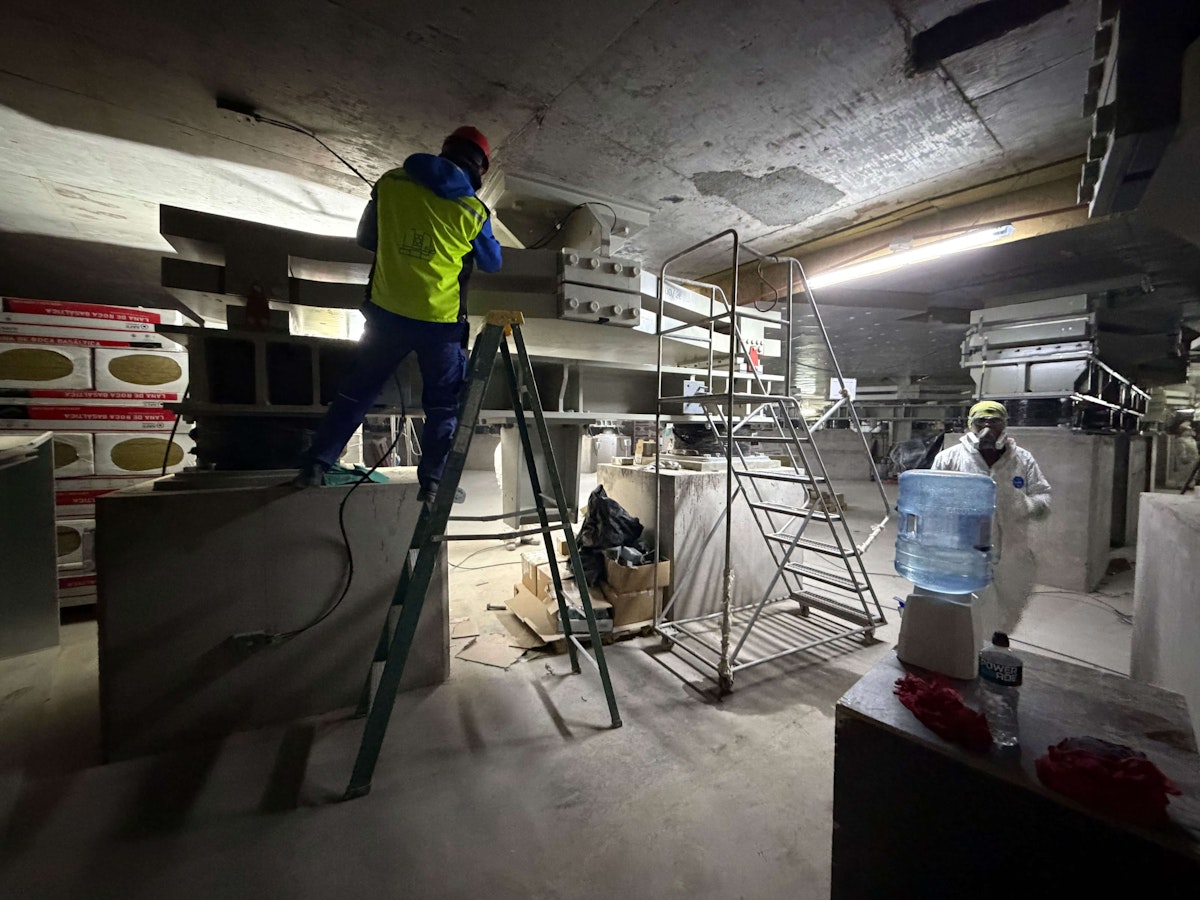
The mission was carried out while the structure was still under construction, before completion, acceptance, and handover to ESO. This created several challenges, including restricted access, limited availability, safety constraints, and difficult site conditions. The area officially remained under the responsibility of the construction company Cimolai. Conditions were especially demanding in the telescope basements, where parallel work, including thermal insulation installation, was still in progress.

The presence of dust and hazardous airborne particles made the installation more difficult. As a result, cable routing could only be temporary and was not straightforward. Nevertheless, we ensured adequate cable lengths throughout the system. Buffer lengths were reserved near the connectors, and the cables were secured to the structure to minimize stress on the sensors.

Figure 10 shows the locations and connection topology of the sensors in the seismic area. The sensors are numbered/named consecutively as they are connected (cables going in and out of each sensor). 

Three sensors are attached (bolted to the concrete) to the ceiling or above the seismic devices, arranged in a triangular, symmetric geometry. In contrast, the other three are bolted exactly below on the bottom side of the isolator devices attached to the ground (see Figure 11). Each sensor axis is locally aligned with the seismic device next to it, looking toward the center of this circular area. 

By knowing exactly the local axis of each sensor aligned to an already well positioned device in such a large area, and from the design geometry, in DewesoftX software one can easily create all necessary mathematics to project the reading of sensors to the pier (and the telescope on top of it) motion in global coordinates (6Dof motion) (see next section for more details). 

From the cabinet in the telescope seismic room, one cable line routes to the basement of the dome. We decided to install the sensors in three different rooms in the auxiliary building (AB), whose locations span a large portion of the enclosure periphery. 

The selected rooms and areas are also of particular interest for monitoring vibration sources affecting those areas. One room accommodates one of the HVAC systems (sensor #7). The other area hosts all water-cooling infrastructure and associated pumps (sensor #8). The 9th sensor is below the oil supply room, with its pumps feeding the telescope axes' hydrostatic bearing system. 

Due to the considerable distances between the cabinet and the initial sensor, as well as between the initial sensor and other sensors within the dome area, we employed two IOLITE repeaters to extend the connection lengths to the affected sensors. The installation commenced with the telescope pier branch, followed by the preparation and connection of each sensor cable. 

After each connection, we verified the state and connectivity in the DewesoftX hardware configuration. Subsequently, we introduced the EtherCAT hub and created a new branch from the telescope area to the dome basement. Similarly, in the dome area, the system’s state was verified by adding a new sensor to the chain. 

Finally, we created the first version of the DewesoftX monitoring displays and widgets, equipped with the necessary live calculations and analysis, such as FFT spectra for all sensors, and commenced data recording. In the next section, we present the data-saving and retention strategy, along with initial results and observations. 

Eyes to the telescope: eyes to the sky 

From the initial analysis of data collected from the sensors, the system’s utility, immense potential, and numerous advantages became evident. The use of highly sensitive, low-noise iolite sensors at low frequencies, where significant dynamical effects of the structure occur, coupled with the robust mathematical and live analysis capabilities of the DewesoftX software, provided a comprehensive understanding of the structure, akin to an open eye on the system. 

We record and store the data locally on an SSD disk, saving only the raw acceleration data from the nine sensors at a 1 kHz rate. With just a click, we can recalculate all mathematical operations and newly created channels from the saved data. 

The software automatically creates data files containing 10 minutes of data, and each file is named based on the local time and date. To save disk space, we used the Dewesoft zip format. 

For analysis, each file can be opened separately or via the multi-file option, depending on the start and stop recording times. For instance, every six hours, a batch of files can be opened quickly, allowing the visualization and analysis of data in one go (a very useful feature). 

With the aforementioned parametrization, each file is approximately 90 megabytes (per 10 minutes). The IPC houses a large RAID 5 hard disk that receives data from the SSD every week, freeing the SSD for new data. Currently, data file access and software control are performed via Windows Remote Desktop over the internal ESO network (from Germany to Chile). 

In the future, we will use Dewesoft Historian to publish the reduced data along with some Key Performance Indicators (KPIs) to a server database. With Historian, the data will be accessible for visualization using dashboards in web clients such as Grafana. In the advanced stages of this project and the observatory database system, we can easily transfer all KPIs to the ESO’s engineering archive. 

Visualizing and collecting data from all sensors is one aspect, but analyzing and interpreting all that data is equally important and should not be overlooked. The key question is how to use and interpret the data collected at different stages of the project. As of now, approximately 3 months of acceleration data, collected 24 hours a day, 7 days a week, have been saved and are available. 

To accurately comprehend data and their interpretations, it’s crucial to examine them from multiple angles. Time- and frequency-domain analysis are instrumental in achieving this. Moreover, converting or filtering accelerations, such as transforming them into velocity and position via time integration, enables scaling information across different frequencies. Given the structure's substantial size and weight and the current phase of the project, we paid special attention to low frequencies. 

Thanks to the strong signal-processing capabilities of DewesoftX, many of the necessary calculations are performed in real time, enabling fast, immediate analysis, visualization, and interpretation. We calculate the velocity and position values online using time-domain analysis tools. In contrast, the Fourier transform, short-time Fourier transform, and rms values in 1/3-octave bands are all available in real time, and we dedicate screens to each view of the signals.

As mentioned earlier, we do not save these newly added channels in the files. Still, we quickly and easily recalculate these for offline analysis, with the option to add new ones or change the calculation parameters, such as the number of FFT points (resolution) and filter frequencies. 

Using the mathematical module, together with the known geometry, the local coordinates of each sensor, and the tri-axial data from the three sensors installed above the pier’s seismic devices, the measured values are projected into the telescope’s six-degree-of-freedom motion in global coordinates.

Alongside the time-domain motion signals, spectra, and RMS values, the data are displayed on a dedicated screen. With real-time information available, the analysis process becomes faster and more intuitive. It is easy to see when a more detailed analysis is needed and which file should be selected for closer examination.

Thanks to this approach, the supporting tools, and the sensors' strong performance, we were able to identify several interesting characteristics of the structure soon after reviewing the results. A detailed analysis is beyond the scope of this paper, but the next section outlines the main preliminary observations.

Live from the basement 

What can we already observe from the sensors installed in the basement of the dome and main structure? In principle, the structure is affected by excitation loads:

• workers moving around during the day and all the machinery they use for their work, 

• wind load, and 

• seismic events. 

The construction site operates daily from 7 a.m. to 7 p.m., and this pattern is clearly reflected in the data. Although the effects of generators, cranes, and other machinery are temporary and linked only to the construction phase, the data still offers valuable insight. It allows us to track how forces are transferred from one part of the structure to another, for example, from the dome area to the telescope pier.

To distinguish short, sporadic events such as hammering, drilling, or workers touching the sensors, we introduced metrics such as crest factor and kurtosis as key performance indicators, supported by visualizations.

Figure 16 presents the measured accelerations from all sensors over a typical night-to-day interval, here from 11 p.m. to 8 a.m. Work and machinery activity begin around 7 a.m. The same figure also shows the averaged FFT for that period, which serves as a signature of the combined environmental and machinery-related effects that emerge early in the morning. At low frequencies, starting at 0.7 Hz, the spectra are dominated by signals from the dome, especially lateral motion in the local x and y directions.

Looking only at the acceleration time signal or the snapshot of the FFT reveals no specific features, but examining the velocities or displacements calculated in the software reveals many interesting features. Figure 17 shows the lateral motions (in µm) during that night together with the rms of velocities (µm/s) expressed in 1/3-octave bands (updated every 10 seconds).

The displacements initially increase and then gradually decrease throughout the night. Additionally, from the spectra and octave analysis, it’s evident that a frequency of approximately 2 Hz predominantly drives the overall motion. This observation is further supported by examining the saved data files, which contain 10 minutes of data and mathematical calculations. Figure 18 illustrates the accelerations, FFT spectra, and lateral displacement of the Dome for 30 seconds, highlighting the dominant motion oscillations around 2Hz. 

The root mean square (rms) velocities, calculated every 10 seconds, are plotted as a function of time (see Figure 19). These curves reveal valuable and intriguing information and trends. They were compared and verified against wind speed and direction data from Cerro Armazones and the Very Large Telescope (VLT) in Paranal, located a few kilometers away. 

Figure 20 displays the wind data recorded that night. A clear correlation between wind changes over time is evident. We have conducted this correlation check over numerous nights and confirmed that the observed motion is related to wind load on the dome structure. 

After several days of data verification, another pattern became clear from the signal color coding. The trend signals cluster into distinct groups. The highest values are associated with the dome’s lateral motion, followed by its vertical motion. Above the isolators, a separate group represents signals from the pier, while the lowest values correspond to measurements at the pier ground level.

This behavior matches our structural expectations and indicates that the telescope is protected from wind loads. During the last couple of months of measurement, the slit doors remained almost closed, with only a small opening of a few meters, and the dome opening faced south, toward the building’s main entrance. This configuration shielded the telescope from northerly winds, as the data also suggests.

Figure 21 shows the time series of the telescope pier 6Dof motion in global coordinates (with the Y axis pointing towards the south), along with their spectra and the rms velocities in 1/3-octave bands. Notably, the amplitude of the pier’s motions is less than 60nm, which is remarkably well-resolved by the sensors. This level is evident from the spectra, which exhibit modes at frequencies as low as 2Hz. 

There were also nights with very strong southwesterly winds. For instance, Figure 22 shows a quite windy night from the 14th to the 15th of February. 

Figure 23 shows the telescope pier 6DoF motions (10 min of data, around 10 PM, see also the amplitude and time in Figure 22) and spectra indicating movements up to 380nm, caused mainly by the wind load on the telescope structure and on the second degree indirectly transmitted from dome reaction forces through the ground. Figure 21 illustrates that we can also appreciate the observation by comparing the amplitudes of the excited modes on this windy night with the measured spectra.

Wind is not the only natural ’shaker’ for the structure, and the site being in a quite active seismic region in the world is permanently excited by earthquakes around it, sometimes hundreds of kilometers away in Chile and Argentina. The system captures seismic effects as small as 2.5 Magnitude on the Richter scale.

We use different ways to correlate the measurement observations with the actual events: either by daily checking national and international seismic research centers, such as Centro Sismológico Nacional, Universidad de Chile, or GFZ Helmholtz-Zentrum für Geoforschung, or first by looking into the live data trends, such as rms velocities, and then confirming the observations by the seismic reports. 

Figure 24 illustrates that, in addition to wind, there were some seismic activities (blue spikes), with one of them exhibiting significantly higher values. The figure also includes a screenshot of the Chilean national seismic site, providing precise information on the time corresponding to the spikes in the data, including the event's location, depth, and magnitude. 

The blue color code corresponds to the RMS values of the telescope’s lateral motion. During earthquakes, this direction experiences the strongest amplification, driven by the pier's lateral modes above the isolation system at around 4.7 Hz.

Often, a simple check of the color pattern and amplitude is enough to distinguish a seismic event from other daytime activities that generate large accelerations or motions. A seismic event also has a global effect on the structure, causing a simultaneous change in the readings of all sensors. This is often visible as a collective increase in RMS velocity, as shown in Figure 25.

The same figure also shows details of a relatively strong nearby earthquake of magnitude 5.3 that occurred at 4:28 a.m. on January 13.

Figure 26 presents the pier’s global motions and their spectra, the dome’s lateral motions, and the Short-time Fourier transform (STFT) of selected signals. The STFT is particularly useful for analyzing non-stationary events, including short-duration or sporadic disturbances such as earthquakes.

During the seismic event that night, the telescope pier exhibited lateral motions of up to 70 µm in the global x- and y-directions, with the strongest responses at 4 Hz and 4.7 Hz. The dome reached lateral motions of up to 21 µm, mainly at 2 Hz.

Such events act as natural excitations of the structure, making them valuable for identifying structural modes and comparing measured behavior with design and simulation results. Measurements collected so far have already helped reveal and confirm several of these design parameters.

Figure 23. Wind from the south and some openings in dome doors: Telescope pier 6DoF motions in µm, 1/3-octave rms velocities in µm/s, and the motion spectra.

Conclusions 

We have introduced the ELT structural vibration monitoring system, using Dewesoft’s low-noise IOLITE 3MEMS sensors, and outlined its architecture and a phased approach, emphasizing its scalability. Recent implementation of the monitoring system on the optical telescope and dome structures showcased the system’s strengths and potential, particularly its ability to capture low-frequency effects and its strong, intuitive live mathematical and analysis tools. 

The project eagerly awaits the results of additional sensor integration into the telescope structure, the implementation of Historian to support long-term trend data, and the availability of data for additional users. Once we equip the telescope structure with a more extensive sensor network, activities such as operational modal analysis (OMA) and vibration level verification can commence. 

Acknowledgments 

We thank and acknowledge the following people for the valuable help and support: M. Mueller, P. Zuluaga, Y. Lammen, G. Jakob, J.C. Gonzales, F. Biancat Marchet, P. Martinez, D. Deiana, G. Vacchia, M. Wallace, S. Solis, A. Wright, J. Dupeyron, P. Barriga, P. Scibior, D. Schneller from ESO, R. Mesar, H. Behmueller, and D. Florjančič from Dewesoft, M. Colussi and his team from Cimolai, and the Airworks engineer team involved in vibration analysis of ELT telescope structure.

References

1. Sedghi, B., Müller, M., and Jakob, G., “E-ELT vibration modeling, simulation, and budgeting,” in [IMCOS15 Integrated Modeling of Complex Optomechanical Systems II (IMC15)], Proc. SPIE (2015). 

2. Adams, D., Fordham, B., Jakob, G. H., MacMartin, D. G., Sedghi, B., Schwartz, D. M., Thompson, H. A., Travouillon, T. D., Smith, B. W., and Kerrian, P., “Management of equipment vibration for extremely large telescopes,” Journal of Astronomical Telescopes, Instruments, and Systems 8(2), 1 – 36 (2022). 

3. Sedghi, B., Müller, M., and Dimmler, M., “Analyzing the impact of vibrations on E-ELT primary segmented mirror,” in [Modeling, Systems Engineering, and Project Management for Astronomy VI], Proc. SPIE 9911 (2016). 

4. Sedghi, B., Zuluaga-Ram´ırez, P., Lampater, U., Pilbauer, D., Leveratto, S., Jakob, G., Müller, M., Abad Pastor, J., Gonzalez-Herrera, J. C., and Patti, S., “ESO ELT - vibration sources characterization: a step forward towards requirement and performance verification,” in [Modeling, Systems Engineering, and Project Management for Astronomy IX], Angeli, G. Z. and Dierickx, P., eds., 11450, 165 – 177, International Society for Optics and Photonics, SPIE (2020). 

5. Sedghi, B., Ramirez, P. Z., Pilbauer, D., Leveratto, S., Lampater, U., Müller, M., Jakob, G., Haug, M., Accardo, M., Lammen, Y., Abad-Pastor, J., and Gonzalez-Herrera, J. C., “ESO ELT: vibration performance and budget verification: measured equipment data as input to telescope model,” in [Modeling, Systems Engineering, and Project Management for Astronomy X], Angeli, G. Z. and Dierickx, P., eds., 12187, 1218714, International Society for Optics and Photonics, SPIE (2022). 

6. Colussi, M., Colussi, L., Ninane, N., Verspecht, J., Sedghi, B., and Müller, M., “Performance analysis overview for the main structure of the Extremely Large Telescope,” in [Modeling, Systems Engineering, and Project Management for Astronomy IX], Angeli, G. Z. and Dierickx, P., eds., 11450, 190 – 214, International Society for Optics and Photonics, SPIE (2020). 

7. Tamai, R., Koehler, B., Cirasuolo, M., Biancat-Marchet, F., Tuti, M., Gonzalez-Herrera, J.-C., and Ramsay, S., “ESO’s ELT halfway through construction,” in [Ground-based and Airborne Telescopes X], Marshall, H. K., Spyromilio, J., and Usuda, T., eds., 13094, 1309415, International Society for Optics and Photonics, SPIE (2024).